A Parallel Genetic Algorithm Approach to the Knife Change Minimisation Problem Aneurin M. Easwaran and Sophia Drossopoulou† Department of Computing, Imperial College, London SW7 2AZ Abstract The knife change minimisation problem is a special case of the Generalised Travelling Salesman Problem arising in the paper industry as a sub-problem to the one-dimensional cutting stock problem. In the knife change minimisation problem a sequence of cutting patterns needs to be produced at a paper machine winder. Each of the patterns consists of a list of reels, the relative position of which can be varied. Thus each pattern gives rise to many permutations. Each knife re-positioning takes time and we therefore seek to minimise the total number of knife changes by determining the sequence of pattern production and which permutation will represent each pattern. A serial genetic algorithm with special crossovers and inversion as mutation was developed to solve the problem. The serial genetic algorithm produces optimal solutions for small problems and improved solutions for medium and large problems. The solutions obtained for instances of any size are of better quality than the solutions obtained in an industrial product, but require longer execution time. Could a distributed genetic algorithm produce better quality solutions for large problems than the serial genetic algorithm? A parallel genetic algorithm based on the serial genetic algorithm was implemented on the Fujitsu AP1000 to answer the question. The results indicate an improvement in the quality of the solutions.
Keywords: Cutting Stock Problem, Parallel Genetic Algorithms, Knife Change Minimisation, Generalised Travelling Salesman Problem
1.
INTRODUCTION AND PROBLEM DESCRIPTION
1.1
Problem Description
The Travelling Salesman Problem (TSP) in its simplest form asks for the shortest route which visits every city exactly once and returns to the initial city. The Generalised TSP (GTSP) [9] asks for the shortest route visiting exactly one city in each and every country.
Figure 1: The Generalised Travelling Salesman Problem
†
Corresponding author; also at
[email protected].
P2-W-1
The GTSP is a difficult optimisation problem with potential applications in the areas of distribution, warehousing and scheduling. The GTSP is clearly NP-hard. One of the applications of a GTSP, occurring in the paper industry, is the knife change minimisation problem: A paper cutting machine (called a winder) is given a number of patterns. Each pattern consists of a collection of reels (or rolls) to be cut, each with a given width. In order to cut these reels, rotary knives on a bar on the winder have to be set to the appropriate positions. The relative position of the reels in each pattern may be changed, resulting in a number of different permutations. After such a permutation is cut, the knives need to be repositioned so as to cut the new widths in the next pattern. The process of knife repositioning takes time, as accuracy of 1 mm or less is required. We therefore want to minimise the number of knife changes needed. We seek to do this by selecting the sequence of production of the patterns and the representative permutation for each pattern. In terms of the GTSP • The patterns correspond to countries. • The permutation of widths in each pattern correspond to the cities. Consider the following example with just three patterns Pattern 1: Pattern 2: Pattern 3:
2, 2, 5, 6 4, 4, 6 2, 3, 8
Two possible solutions are given below: Solution A - 11 Knife Changes
Solution B - 8 Knife Changes
8
2
2
6
4
3
2
4
5
6
Figure 2: Two Solutions to a Small Knife Change Minimisation Problem
For solution A the knives have to be positioned first at 0, 5, 11, 13 and 15 and then at 6, 10, and 14 and then at 8, 11 and 13. The number of knife changes required for Solution A is 11. For solution B the knives have to be positioned first at 0, 8, 10 and 13 and then at 2 and 15 and then at 4 and 14. The number of knife changes required for Solution B is 8. Therefore, solution B is better than solution A. Note that, as defined here, the knife change minimisation problem is an asymmetric GTSP: setting a knife requires measurement, whereas removing it does not. The number of possible solutions grows exponentially with number of patterns and number of widths per pattern. In general, the number of possible solutions for a problem is: n! x m1 x m2 x ... x mn where n is the number of patterns and mi is the number of width permutations in pattern i. If pattern i contains ki distinct widths, mi = ki!. Typical real-world problems give rise to numbers in the range of 1030-1080. This is because a “typical” problem may have 10-30 patterns, each of
P2-W-2
which may have 3-10 reels. The number of solutions for the small example above is: 3! x
4! 3! x x 2 2
3! = 1386.
The remainder of this paper is organised as follows: Section 2 provides an overview of serial and parallel genetic algorithms. Section 3 presents the application of parallel genetic algorithms to the knife change minimisation problem. Section 4 documents the assessment of the parallel genetic algorithm. Section 5 contains the conclusion.
2.
GENETIC ALGORITHMS
Over the past few years genetic algorithms have attracted a lot of attention in Computer Science and AI. They have been applied, among others to combinatorial optimisation problems, for example the TSP [19], the job-shop scheduling problem [7] and the bin-packing problem [12].
2.1
Serial Genetic Algorithms
Genetic algorithms [11] manipulate a population of individual string structures, each with an associated value of fitness. A new generation of the population is created by probabilistically selecting individuals from the population on the basis of their fitness. The genetic operation selection is based on the Darwinian principle of reproduction and survival of the fittest. The selection is done in such a way that the better an individual’s fitness, the more likely it is to be selected. The genetic operation of crossover is applied on pairs of selected individuals to create new individuals and to test new points in the search space. The operation of crossover starts with two parents and produces two offspring. Each offspring contains some genetic material from each of its parents. The genetic operation of mutation is used to restore genetic diversity that may be lost in a population. The operation of mutation is applied on a selected individual. A random point is selected on the individual and the single character at that point in randomly changed. Mutation is used very sparingly in most genetic algorithm applications. A typical genetic algorithm [11] is presented below: 1. Randomly generate a population of M structures S(0) = {s(1, 0), ... , s(M, 0)}. 2. For each new string s(i, t) in S(t), compute and save its fitness value using the fitness measure f(s(i, t)). 3. For each s(i, t) in S(t) compute the selection probability defined by f ( s( i, t )) p( i , t ) = ∑ f ( s( i, t )) i
4. Generate a new population S(t + 1) by applying the following three genetic operators on S(t). The genetic operations are applied to individual strings in the population selected using the selection probability defined. i) Reproduce an existing individual string by copying it into the new population. ii) Create two new strings from two existing by genetically recombining substrings using the crossover operation at a randomly chosen crossover point. iii) Create a new string from an existing string by randomly mutating the character at one randomly chosen position in the string. 5. If an appropriate stopping criterion fails, go to 2. P2-W-3
2.2
Parallel Genetic Algorithms
In the past few years, parallel genetic algorithms have been used to solve difficult problems. Hard problems need bigger population and this translates directly into higher computational costs. The basic motivation behind many early studies of parallel genetic algorithms was to reduce the processing time needed reach an acceptable solution. This was accomplished by implementing genetic algorithms on different parallel architectures. In this paper we present our results which indicate that parallel genetic algorithms find better solutions than the comparably sized serial genetic algorithms. Today, the study of parallel genetic algorithms is flourishing. However, most of the research has been empirical and, until recently, we lacked a theory that helped resolve the fundamental questions that arise in the design of these algorithms[2]. Cantu-Paz [2] presents four different ways to parallelise genetic algorithms. The first approach in parallelising genetic algorithms is to do a global parallelisation, whereby the evaluation of individuals and the application of genetic operators are explicitly parallelised. Every individual has a chance to mate with all the rest (i.e., there is random mating). Therefore, the semantics of the genetic operators remain unchanged. This method is relatively easy to implement and a speedup proportional to the number of processors can be expected. A more sophisticated idea is used in coarse grained parallel genetic algorithms, whereby the population is divided into a few subpopulations which are relatively isolated from each other. This model of parallelisation introduces a migration operator that sends some individuals from one subpopulation to another. Two population genetics models for population structures are used in different implementations of coarse grained genetic algorithms: the island model and the stepping stone model. The population in the island model is partitioned into small subpopulations by geographic isolation and individuals can migrate to any other subpopulation. In the stepping stone model, the population is partitioned in the same way, but migration is restricted to neighbouring subpopulations. Both models have been used in parallel genetic algorithms. Sometimes coarse grained genetic algorithms are known as ‘distributed’ genetic algorithms since they are usually implemented in distributed memory MIMD (multiple instruction multiple data) machines. The third approach in parallelising genetic algorithms uses fine grained parallelism, whereby the population is partitioned into a large number of very small subpopulations. The ideal case is to have just one individual for every processing element available. This model calls for massively parallel computers. In the last two approaches, selection and mating occur only within each subpopulation. Based on this, the term deme is borrowed from Biology to refer to a subpopulation. The fourth approach uses some combination of the first three methods, and this is called hybrid parallel genetic algorithms. One way to hybridise a parallel genetic algorithm is to use global parallelisation on each of the demes of a coarse grained genetic algorithm.
3. PARALLEL GENETIC ALGORITHMS AND THE KNIFE CHANGE MINIMISATION PROBLEM This section describes the representation and genetic operators used for the knife change minimisation problem.
3.1
Individual Representation
Individuals are sequences of pattern permutations, i.e., candidate solutions. If we represented individuals in terms of a single chromosome, we would need to take extra care to prevent the mutation and the crossover operators from creating individuals which do not belong to the P2-W-4
solution space. For example, the mutation operator must only be applied on the widths within a pattern or across whole patterns only. Performance of the algorithm would be very poor with a single chromosome representation because of the extra care required to prevent genetic operators from creating illegal individuals. Therefore, as in [1], we decided to use a two-level representation of an individual using two chromosomes. We represent an individual in the following manner: • Route chromosome: represents the sequence in which patterns are visited. • Pattern chromosome: contains all the widths in the each pattern and thus represents the width permutation of each pattern. • Pattern Boundary: is used to identify the start and end of each pattern in the structured Pattern Chromosome. Pattern Boundary is not affected by mutation or crossover operation. Consider again the example from section 1.1 - solution A would be represented as: Route Chromosome
1 2
3
Pattern Chromosome
5 6
2 2
Pattern Boundary
6 4
4
8 3
2
4 7 10
Figure 3: Individual Representation
3.2
Genetic Operators
Illegal pattern sequences or width permutations would be produced if the classical genetic operators devised by Holland [10] were applied without adaptation. For our purposes, the genetic operators need to preserve the following properties: 1. the route chromosome is a permutation of numbers 1..n (for n patterns), 2. each pattern in the pattern chromosome represents a permutation of the original pattern. The constraints raise the requirement for mutation/crossover operations that preserve the permutation property. Furthermore, we need to constrain the mutation/crossover operations so that they do not apply further than the boundaries defined by the Pattern Boundary.
3.2.1
Crossovers
These crossovers start with two permutations of a set as parents and produce two offspring which are permutations of the same set. The Order Crossover The order crossover [4 & 5] consists of four stages. The stages are explained in terms of an example: Stage 1 - Starting with strings A and B which are permutations of 1 to 10, we select a matching section, denoted by ...|...|.... A = 9 8 4 | 5 6 7 | 1 3 2 10 B = 8 7 1 | 2 3 10 | 9 5 4 6
P2-W-5
Stage 2 - Each string maps to constituents of the matching section. When string B maps to string A, the values 5, 6 and 7 will leave holes (marked by H) in the string: B = 8 H 1 | 2 3 10 | 9 H 4 H
Stage 3 - These holes are filled with a sliding motion that starts following the second crossing site. B = 2 3 10 H H H 9 4 8 1
Stage 4 - The holes are filled with the matching section values taken from the mate. Performing this operation and completing the complementary cross we obtain the offspring A ′ and B ′ as follows: A ′ = 5 6 7 | 2 3 10 | 1 9 8 4 B ′ = 2 3 10 | 5 6 7 | 9 4 8 1 The Cycle Crossover The cycle crossover [16] performs recombination under the constraint that each value comes from one parent or the other. To illustrate this, we consider an example A = 9 8 2 1 7 4 5 10 6 3 B = 1 2 3 4 5 6 7 8 9 10
Instead of choosing crossover points, we start at any point and choose a value from the first parent. In this case we choose 1: A′ = - - - 1 - - - - - We want every value to be taken from one of the two parents. The choice of value 1 from string A means that we must now get value 4 from string A because of the 4 in position 4 of string B. A′ = - - - 1 - 4 - - - This selection in turn requires that we select value 6 from string A. This process continues until we are left with the following values: A′ = 9 - - 1 - 4 - - 6 The selection of a 9 means that we should now choose a 1 from string A; however, this is not possible; a 1 having been selected as the first value. We eventually return to the value of origin thus completing a cycle; this gives the operator its name. Following the completion of the first cycle, the remaining values are filled from the opposite strings. Completing the example and performing the complimentary cross yields the following children tours: A ′ = 9 2 3 1 5 4 7 8 6 10 B ′ = 1 8 2 4 7 6 5 10 9 3
3.2.2
Mutation
Inversion is a mutation operator that produces legal pattern sequences or width permutations as offspring. Under inversion two points are chosen along the length of the chromosome, the chromosome is cut at those points, and the substring between those points is inverted:
P2-W-6
1
2
3
4
5
6
7
8
9 10
1
2
7
6
5
4
3
8
9 10
Figure 4: Mutation process
3.2.3
Selection
Roulette Wheel Selection The roulette wheel selection [8] is a linear search through a roulette wheel with slots weighted in proportion to individual fitness values. To do this, the partial sum of the fitness value of each individual in a population is accumulated in a variable and for each individual it is stored in a weighted roulette wheel. Then a loop searches through the weighted roulette wheel until the partial sum is greater than or equal to a value calculated by multiplying the sum of the population fitnesses by a pseudorandom number. The last individual to contribute to the partial sum is selected. For example, consider a population with five individuals: Individual
Fitness
Weighted Roulette Wheel
Individual1
0.6
Partial Sum = 0.6
Individual2
0.2
Partial Sum = 0.8
Individual3
0.4
Partial Sum = 1.2
Individual4
0.6
Partial Sum = 1.8
Individual5
0.3
Partial Sum = 2.1
Total fitness of the population is 2.1, for a pseudorandom number = 0.682, the search value will be 0.682 x 2.1 = 1.4. The partial sum 1.8 is the first one greater than 1.4. Thus, the individual to be selected is Individual4. Tournament Selection The tournament selection selects two individuals using the roulette wheel selection method and then picks the fittest of these two. Random Selection The random selection method randomly selects an individual from the population. A way to do this is to generate a pseudorandom number, multiply the size of the population by the generated number and select the corresponding individual. For example, for a pseudorandom number 0.519 and size of population 100, the random individual will be 100 x 0.519 = 51.9. Therefore, individual 52 is selected from the population.
P2-W-7
3.3
Tuning the Genetic Search
Heuristics were developed to improve the performance of the genetic algorithm:
3.3.1
Route Repair Heuristic
This classical two-exchange scheme (see [14]) is best illustrated by an example:
P1
P2
P1
P2
P4
P3
P4
P3
Figure 5: Route repair
3.3.2
Pattern Repair Heuristic
This heuristic takes a pair of adjacent patterns in a route, and maximises commonality of knife settings from the left hand edge by finding all widths in the second pattern which must equal the widths on the left edge of the first pattern. For example, (5-3-2), (4-3-5) would become (5-3-2), (5-3-4).
3.4
Implementation and Underlying Problems
Coarse grained parallel genetic algorithms are the most popular model and have been applied to many applications (e.g. [17], [13] and [15]). A coarse grained parallel genetic algorithm was developed to solve the knife change minimisation problem on the Fujitsu AP1000. Coarse grained parallel genetic algorithms are also known as ‘distributed genetic algorithms’ and are usually implemented on distributed memory MIMD machines (e.g. Fujitsu AP1000). In the coarse grained parallel genetic algorithm, the population is divided into a few subpopulations which are relatively isolated from each other. This model of parallelisation introduces a migration operator that is used to send some individuals from one subpopulation to another. The population genetic model chosen was the stepping stone model. In the stepping stone model, the migration is restricted to neighbouring subpopulations. The stepping stone model was chosen because it closely resembles the torus topology of the AP1000. Using the stepping stone model or island model would not make any difference to the quality of solutions obtained because the initial population is random. The size of the population affects the performance of the genetic algorithm. Therefore the size and number of demes must be determined with care. Once the size and number of demes is determined then one has to establish how they are going to communicate. Migration is a very complex operator and is affected by the following parameters : • Migration interval. Intuitively, migration should occur after good individuals are built - the
average fitness of the population is above a particular threshold. Migrating before that is probably a waste of (communication) resources. • Migration rate. The number of individuals that should migrate is very closely related with the
migration interval. If individuals are developed, maybe good results can be obtained by migrating just a few. • Topology. If a topology with a long diameter is used, good solutions take longer time to
propagate to all the demes. P2-W-8
4.
ASSESSMENT OF THE PARALLEL GENETIC ALGORITHM
The parallel genetic algorithm is built on the serial genetic algorithm [6] which produces better quality solutions than an industrial product. The serial genetic algorithm was tuned (selecting the best genetic operators and crossover and mutation rates) to obtain good performance (see [6]). Therefore the parallel genetic algorithm required no further tuning except selecting a good migration interval and topology to achieve good performance. The parallel genetic algorithm has the following features : •
Tournament selection.
•
Cycle crossover.
•
A random initial population with 100 individuals and the number of generations is 100.
•
Crossover rate - Route chromosome : 70% and Pattern chromosome : 90%.
•
Mutation Rate - Route chromosome : 30% and Pattern chromosome : 10%.
•
Elitist Model - Preserving the best individual in every generation.
•
Repair heuristic applied to all individuals in the last two generations.
Migration between cells is controlled by three parameters : topology, migration rate and migration interval. The topology used in this part of the assessment is a 2 x 2 Torus network and the migration rate is one (i.e. only the best individual is sent to the neighbours). Different migration intervals were experimented and the results are tabulated below for five problems of varying sizes. The size of a problem is equal to the number of possible solutions. The results for the various migration intervals are compared with the results produced with no migration (No Mig.). The values in the table below for each problem is the average number of knife changes calculated after ten replicate runs. AAAA AAAA AAAA AAAA AAAA AAAA AAAA AAAA AAAAAAAAAAAAAAAAAAAA AAAAAAAAAAAAAAAAAAAA AAAAAAAAAAAAAAAAAAAA AAAAAAAAAAAAAAAAAAAA AAAAAAAAAAAAAAAAAAAA AAAAAAAAAAAAAAAAAAAA AAAAAAAAAAAAAAAAAAAA AAAA AAAA AAAA AAAA AAAA AAAA AAAA AAAA AAAA Problem AAAA AAAA Every AAAA Every 5th AAAAEvery 10th AAAA AAAA AAAA No Every 25th Every 50th AAAA AAAA AAAA AAAA AAAA AAAA AAAA AAAA AAAA AAAA AAAA AAAA AAAA AAAA AAAA AAAA AAAA AAAA AAAA AAAA AAAA AAAA AAAA AAAA AAAA AAAAMigration AAAA AAAAGeneration AAAAGeneration AAAA AAAA AAAA Size Generation Generation Generation AAAA AAAA AAAA AAAA AAAA AAAA AAAA AAAA AAAA AAAA AAAA AAAA AAAA AAAA AAAA AAAA AAAAAAAAAAAAAAAAAAAA AAAA AAAAAAAAAAAAAAAAAAAA AAAA AAAAAAAAAAAAAAAAAAAA AAAA AAAA AAAAAAAAAAAAAAAAAAAA AAAAAAAAAAAAAAAAAAAA AAAA AAAAAAAAAAAAAAAAAAAA AAAA AAAAAAAAAAAAAAAAAAAA AAAA AAAA 15 AAAA6.05 x 10 AAAA AAAA AAAA AAAA AAAA AAAA AAAA AAAA AAAA AAAA AAAA AAAA AAAA AAAA AAAA 18 20 21 18 18 18 AAAA AAAA AAAA AAAA AAAA AAAA AAAA AAAA AAAA AAAA AAAA AAAA AAAA AAAA AAAA AAAA AAAAAAAAAAAAAAAAAAAA AAAA AAAAAAAAAAAAAAAAAAAA AAAA AAAAAAAAAAAAAAAAAAAA AAAA AAAA AAAAAAAAAAAAAAAAAAAA AAAAAAAAAAAAAAAAAAAA AAAA AAAAAAAAAAAAAAAAAAAA AAAA AAAAAAAAAAAAAAAAAAAA AAAA AAAA 38 AAAA AAAA AAAA AAAA AAAA AAAA AAAA AAAA AAAA7.87 x 10 AAAA AAAA AAAA AAAA AAAA AAAA AAAA 47 46 44 44 44 44 AAAA AAAA AAAA AAAA AAAA AAAA AAAA AAAA AAAA AAAA AAAA AAAA AAAA AAAA AAAA AAAA AAAAAAAAAAAAAAAAAAAA AAAA AAAAAAAAAAAAAAAAAAAA AAAA AAAAAAAAAAAAAAAAAAAA AAAA AAAA AAAAAAAAAAAAAAAAAAAA AAAAAAAAAAAAAAAAAAAA AAAA AAAAAAAAAAAAAAAAAAAA AAAA AAAAAAAAAAAAAAAAAAAA AAAA AAAA AAAA AAAA AAAA AAAA AAAA AAAA AAAA 39 AAAA AAAA3.04 x 10 AAAA AAAA AAAA AAAA AAAA AAAA AAAA 64 62 62 60 60 60 AAAA AAAA AAAA AAAA AAAA AAAA AAAA AAAA AAAA AAAA AAAA AAAA AAAA AAAA AAAA AAAA AAAAAAAAAAAAAAAAAAAA AAAA AAAAAAAAAAAAAAAAAAAA AAAA AAAAAAAAAAAAAAAAAAAA AAAA AAAA AAAAAAAAAAAAAAAAAAAA AAAAAAAAAAAAAAAAAAAA AAAA AAAAAAAAAAAAAAAAAAAA AAAA AAAAAAAAAAAAAAAAAAAA AAAA AAAA AAAA AAAA AAAA AAAA AAAA AAAA AAAA AAAA 52 AAAA5.28 x 10 AAAA AAAA AAAA AAAA AAAA AAAA AAAA 67 66 66 65 65 65 AAAA AAAA AAAA AAAA AAAA AAAA AAAA AAAA AAAA AAAA AAAA AAAA AAAA AAAA AAAA AAAA AAAAAAAAAAAAAAAAAAAA AAAA AAAAAAAAAAAAAAAAAAAA AAAA AAAAAAAAAAAAAAAAAAAA AAAA AAAA AAAAAAAAAAAAAAAAAAAA AAAAAAAAAAAAAAAAAAAA AAAA AAAAAAAAAAAAAAAAAAAA AAAA AAAAAAAAAAAAAAAAAAAA AAAA AAAA AAAA AAAA AAAA AAAA AAAA AAAA AAAA 72 AAAA AAAA4.82 x 10 AAAA AAAA AAAA AAAA AAAA AAAA AAAA 88 88 87 87 85 85 AAAA AAAA AAAA AAAA AAAA AAAA AAAA AAAA AAAA AAAA AAAA AAAA AAAA AAAA AAAA AAAA AAAAAAAAAAAAAAAAAAAA AAAA AAAAAAAAAAAAAAAAAAAA AAAA AAAAAAAAAAAAAAAAAAAA AAAA AAAA AAAAAAAAAAAAAAAAAAAA AAAAAAAAAAAAAAAAAAAA AAAA AAAAAAAAAAAAAAAAAAAA AAAA AAAAAAAAAAAAAAAAAAAA AAAA AAAA
The results presented above indicate that good solutions are obtained when the migration interval is greater than or equal to ten generations. Better solutions are obtained when the migration intervals are larger because individuals are developed between each migration. The execution time is lesser when the migration intervals are larger because less time is spent on communication between processors and synchronisation of processors. We found that creating an entire new population with the migrated individuals lead to better quality solutions than a new population created with migrated individuals and individuals from the old population. Migrating the best individuals often does not facilitate the development of individuals and the diversity of the population is minimal as the population is built with the best individuals migrated.
P2-W-9
The table below shows the effect on the quality of solution when the number of processors are varied in the torus topology. For each problem two results are given - the first number is the average number of knife changes when the population size and the number of generations is equal to hundred and the second number is the average number of knife changes when the population size and the number of generations is equal to fifty. The average number of knife changes for each problem is calculated after ten replicate runs. The serial genetic algorithm and the parallel genetic algorithm have the same features - elitism, cycle crossover, tournament selection, random initial population and repair in the last two generations. The migration interval is ten generations and the migration rate is one for the parallel genetic algorithm. AAAA AAAA AAAA AAAA AAAA AAAA AAAA AAAA AAAA AAAA AAAA Serial GA AAAA 2 x 2 Torus AAAA 4 x 4 Torus AAAA 8 x 8 Torus AAAA 10 x 10 Torus AAAA AAAA AAAA AAAA AAAA AAAA AAAA AAAA AAAA AAAA AAAA AAAA AAAA AAAA AAAA AAAA AAAAAAAAAAAAAAAAAAAAAAAA AAAAAAAAAAAAAAAAAAAAAAAA AAAA AAAAAAAAAAAAAAAAAAAAAAAA AAAAAAAAAAAAAAAAAAAAAAAA AAAAAAAAAAAAAAAAAAAAAAAA AAAAAAAAAAAAAAAAAAAAAAAA 15 AAAA AAAA AAAA AAAA AAAA AAAA AAAA AAAA 6.05 x 10 AAAA AAAA AAAA AAAA AAAA AAAA 18.4 18 18 18 18 AAAA AAAA AAAA AAAA AAAA AAAA AAAA AAAA AAAA AAAA AAAA AAAA AAAA AAAA AAAA AAAA AAAA AAAA AAAA AAAA AAAA AAAA AAAA AAAA AAAA AAAA AAAA AAAA AAAA AAAA AAAA AAAA AAAA AAAA AAAA 19.4 19 18 18 18 AAAA AAAA AAAA AAAA AAAA AAAA AAAA AAAA AAAA AAAA AAAA AAAA AAAA AAAA AAAA AAAA AAAA AAAA AAAA AAAA AAAA AAAAAAAAAAAAAAAAAAAAAAAA AAAAAAAAAAAAAAAAAAAAAAAA AAAAAAAAAAAAAAAAAAAAAAAA AAAAAAAAAAAAAAAAAAAAAAAA AAAAAAAAAAAAAAAAAAAAAAAA AAAAAAAAAAAAAAAAAAAAAAAA AAAA AAAA AAAA AAAA AAAA AAAA AAAA AAAA 7.87 x 1038 AAAA AAAA AAAA AAAA AAAA AAAA 46.7 44 44 44 44 AAAA AAAA AAAA AAAA AAAA AAAA AAAA AAAA AAAA AAAA AAAA AAAA AAAA AAAA AAAA AAAA AAAA AAAA AAAA AAAA AAAA AAAA AAAA AAAA AAAA AAAA AAAA AAAA AAAA AAAA AAAA AAAA AAAA AAAA AAAA 48.2 46 45 45 45 AAAA AAAA AAAA AAAA AAAA AAAA AAAA AAAA AAAA AAAA AAAA AAAA AAAA AAAA AAAAAAAAAAAAAAAAAAAAAAAA AAAA AAAAAAAAAAAAAAAAAAAAAAAA AAAA AAAA AAAAAAAAAAAAAAAAAAAAAAAA AAAAAAAAAAAAAAAAAAAAAAAA AAAA AAAAAAAAAAAAAAAAAAAAAAAA AAAA AAAAAAAAAAAAAAAAAAAAAAAA AAAA AAAA AAAA AAAA AAAA AAAA AAAA AAAA AAAA 39 AAAA 3.04 x 10 AAAA AAAA AAAA AAAA AAAA AAAA 63.8 60 60 60 60 AAAA AAAA AAAA AAAA AAAA AAAA AAAA AAAA AAAA AAAA AAAA AAAA AAAA AAAA AAAA AAAA AAAA AAAA AAAA AAAA AAAA AAAA AAAA AAAA AAAA AAAA AAAA AAAA AAAA AAAA AAAA AAAA AAAA AAAA AAAA 69.8 62 62 62 62 AAAA AAAA AAAA AAAA AAAA AAAA AAAA AAAA AAAA AAAA AAAA AAAA AAAA AAAA AAAAAAAA AAAA AAAA AAAA AAAA AAAA AAAA AAAA AAAA AAAA AAAA AAAA AAAA AAAA AAAA AAAA AAAA AAAA AAAA AAAA AAAA AAAA AAAA AAAA AAAA AAAA AAAA AAAA AAAA AAAA AAAA AAAA AAAA AAAA AAAA AAAAAAAAAAAA52AAAAAAAA AAAAAAAAAAAAAAAAAAAA AAAAAAAAAAAAAAAAAAAAAAAAAAAAAAAAAAAAAAAAAAAA AAAAAAAAAAAAAAAAAAAA AAAAAAAAAAAAAAAAAAAA AAAA AAAA AAAA AAAA AAAA AAAA AAAA AAAA AAAA AAAA AAAA AAAA 5.28 x 10 66.2 65 65 63 62 AAAA AAAA AAAA AAAA AAAA AAAA AAAA AAAA AAAA AAAA AAAA AAAA AAAA AAAA AAAA AAAA AAAA AAAA AAAA AAAA AAAA AAAA AAAA AAAA AAAA AAAA AAAA AAAA AAAA AAAA AAAA AAAA AAAA AAAA AAAA 70.6 70 68 65 65 AAAA AAAA AAAA AAAA AAAA AAAA AAAA AAAA AAAA AAAA AAAA AAAA AAAA AAAA AAAA AAAA AAAA AAAA AAAA AAAA AAAA AAAAAAAAAAAAAAAAAAAAAAAA AAAAAAAAAAAAAAAAAAAAAAAA AAAAAAAAAAAAAAAAAAAAAAAA AAAAAAAAAAAAAAAAAAAAAAAA AAAAAAAAAAAAAAAAAAAAAAAA AAAAAAAAAAAAAAAAAAAAAAAA AAAA AAAA AAAA AAAA AAAA AAAA AAAA 72 AAAA AAAA AAAA AAAA AAAA AAAA AAAA 4.82 x 10 AAAA AAAA AAAA AAAA AAAA AAAA AAAA 87.9 87 85 83 83 AAAA AAAA AAAA AAAA AAAA AAAA AAAA AAAA AAAA AAAA AAAA AAAA AAAA AAAA AAAA AAAA AAAA AAAA AAAA AAAA AAAA AAAA AAAA AAAA AAAA AAAA AAAA AAAA AAAA AAAA AAAA AAAA AAAA AAAA AAAA 90.2 90 88 88 84 AAAA AAAA AAAA AAAA AAAA AAAA AAAA AAAA AAAA AAAA AAAA AAAA AAAA AAAA AAAAAAAAAAAAAAAAAAAAAAAA AAAA AAAAAAAAAAAAAAAAAAAAAAAA AAAA AAAA AAAAAAAAAAAAAAAAAAAAAAAA AAAAAAAAAAAAAAAAAAAAAAAA AAAA AAAAAAAAAAAAAAAAAAAAAAAA AAAA AAAAAAAAAAAAAAAAAAAAAAAA AAAA AAAA
Problem Size
The results indicate that the parallel genetic algorithm finds better quality solutions (greater than 6% improvement for large problems when the population size and the number of generations is equal to hundred) than the serial genetic algorithm. The execution time is much lesser and the improvement in the quality of the solution is greater (improvement of 7%) with the parallel genetic algorithm when the population size and the number of generations is equal to fifty. The quality of the solution improves and the execution time remains the same as the number of processors increase. The improvement in the quality of the solution is due to more processors working on the same problem. Cohoon et al. [3] in their experiments found that the parallel genetic algorithm with migration outperformed both a parallel genetic algorithm without migration and a serial genetic algorithm.
5.
CONCLUSION
The parallel genetic algorithm for the knife change minimisation problem produces better quality solutions than the serial genetic algorithm. The improvement in the quality of solution is due to the migration operator in the parallel genetic algorithm but it also responsible for increasing the execution time of the algorithm. It is clear that much remains to be done in terms of improving the quality of the solution. Our future work will concentrate on : •
Generating a variety of initial populations on various processors. Presently the parallel genetic algorithm works with a random initial population. Heuristics will be used to generate improved initial population [6].
•
Varying the migration rate. Migrating a variety of individuals and not just the best one. Tanese [18] found that migrating too many individuals too frequently or too few individuals very frequently degraded the performance of the algorithm. P2-W-10
The purpose of parallelising the genetic algorithm was to investigate whether the quality of the solution would improve if a distributed genetic algorithm is used to solve the knife change minimisation problem - the results show an improvement in the quality of the solution with the parallel genetic algorithm and thus indicate an improvement in the quality of the solution if a distributed genetic algorithm is used.
P2-W-11
6.
REFERENCES
[1] J. Alexopoulos, Routing and Scheduling of Network Request Using Genetic Algorithms, MSc Thesis, Department of Computing, Imperial College, London 1995 [2] E. Cantu-Paz, A Summary of Research on Parallel Genetic Algorithms, Illinois Genetic Algorithm Laboratory, University of Illinois at Urbana-Champaign, 1995 [3] J. Cohoon, S. Hegde, W. Martin and D. Richards, Punctuated Equilibria : A Parallel Genetic Algorithm, In John J. Grefenstette, editor, Proceedings of the Second International Conference on Genetic Algorithms, Lawrence Erlbaum Associates, 1987 [4] L. Davis, Applying adaptive algorithms to epistatic domains, Proceedings of the 9th International Joint Conference on Artificial Intelligence, (pp 162-164), 1985 [5] L. Davis, Job shop scheduling with genetic algorithms, Proceedings of an International Conference on Genetic Algorithms and Their Applications, (pp 136-140), Ed. J. Grefenstette, Lawrence Erlbaum Associates, Hillsdale, NJ., 1985 [6] A. M. Easwaran, S. Drossopoulou and C. Goulimis, A Genetic Algorithm Approach to the Knife Change Minimisation Problem, Submitted for Publication, Department of Computing, Imperial College, 1996, Report Number 16/96 [7] H. Fang, P. Ross and D. Corne, A Promising Genetic Algorithm Approach to Job-Shop Scheduling, Rescheduling and Open-Shop Scheduling Problems, Proceedings of the Fifth International Conference on Genetic Algorithms, S. Forrest (ed.), San Mateo: Morgan Kaufmann, 1993, (pp 375 - 382) [8] D. E. Goldberg, Genetic Algorithms in Search, Optimization and Machine Learning, Addison Wesley, 1989 [9] A. L. Henry-Labordere, The Record Balancing Problem: A Dynamic Programming Solution of a Generalised Travelling Salesman Problem, RIRO B-2, 1969, (pp 43 - 49) [10] J. H. Holland, Adaptation in Natural and Artificial Systems, Ann Arbor: University of Michigan Press, 1975 [11] A. J. Jones, Models of living systems: Evolution and Neurology, To be published, Dept. of Computing, Imperial College, London, 1995 [12] S. Khuri, M. Schutz, and J. Heitkotter, Evolutionary Heuristics for the Bin Packing Problem, Proceedings of the International Conference on Artificial NNs and GAs, Apr. 1995, (pp 18 - 21) [13] D. Levine, A Parallel Genetic Algorithm for the Set Partitioning Problem, PhD Thesis, Illinois Institute of Technology, 1994 [14] S. Lin, Computer Solutions of the Travelling Salesman Problem, Bell System Tech. J. 44, (pp. 2245 - 2269), 1965 [15] H. Mühlenbein, Parallel Genetic Algorithms, Population Genetics and Combinatorial Optimization, In Proceedings of the Third International Conference on Genetic Algorithms, Morgan Kaufmann Publishers, 1989 [16] I. M. Oliver, D. J. Smith, and J. R. C. Holland, A study of permutation crossover operators on the travelling salesman problem, Proceedings of the Second International Conference on Genetic Algorithms and Their Applications, (pp. 224 -230), 1987 [17] T. Strarkweather, D. Whitley and K. Mathias, Optimization Using Distributed Genetic Algorithms, In H. P. Schwefel and R. Männer, editors, Parallel Problem Solving from Nature P2-W-12
Proceedings of 1st Workshop, PPSN 1, Volume 496 of Lecture Notes in Computer Science, pages 176 - 185, Berlin, Germany: Springer-Verlag, 1991 [18] R. Tanese, Distributed Genetic Algorithms, In J. D. Schaffer, editor, Proceedings of the Third International Conference on Genetic Algorithms, Morgan Kaufmann Publishers, 1989 [19] C. L. Valenzuela, Evolutionary Divide and Conquer: A novel genetic approach to the TSP, PhD Thesis, Department of Computing, Imperial College, London, 1995
P2-W-13