Moreover, in case of video coding of very high motion scenes, the number of Intra ...... [7] Orinoco: http://www.chipvision.com/orinoco/index.php. [8] T. Wiegand ...
A Parallel Approach for High Performance Hardware Design of Intra Prediction in H.264/AVC Video Codec Muhammad Shafique, Lars Bauer, and Jörg Henkel University of Karlsruhe, Chair for Embedded Systems, Karlsruhe, Germany {shafique, lars.bauer, henkel} @ informatik.uni-karlsruhe.de
I.
These multiple Intra Prediction modes also significantly improve the compression ratio of an H.264 Intra Frame Codec that targets high-end encoding applications, e.g. digital cinema etc. An alternative in this case is the MJPEG20002 [2] that uses Discrete Wavelet Transforms (DWT) and Arithmetic Coding. Several studies (e.g. [10], [13]) show that H.264 Intra Prediction modes outperform MJPEG 2000 in terms of both subjective (visual appearance) and objective (Peak Signal to Noise Ratio, PSNR) video quality. Ref. [13] shows that H.264 Intra gives 0.1–1.8 dB3 better PSNR than JPEG2000. The ratio of the decoder complexities for JPEG, JPEG2000, and H.264 Intra Frame Codec is about 1:10:2. Better quality and reduced complexity make H.264 Intra Frame Codec a more attractive solution for high-end applications than MJPEG2000. Moreover, due to its blockbased processing, H.264 is more hardware-friendly.
an MB with minimum block distortion, i.e. Sum of Absolute Differences (SAD)
978-3-9810801-5-5/DATE09 © 2009 EDAA
80%
Scene with Very High Motion
70% 60% 50%
Scene with Mediumto-Slow Motion
40% 30% 20%
Scene with High-toMedium Motion
10% 0% 1
21
41
61
81
101
121
141
161
181
201
221
241
261
281
301
Frame Number
Fig. 1: Distribution of I-MBs in Slow-to-Very-High Motion Scenes (Test Conditions: IPPP…, CAVLC, QP=28, 30fps)
Summary: Intra Prediction is the major processing bottleneck when considering: a) Intra Frame Coder for high-end encoding applications and b) hectic motion scenes with high number of I-MBs. Intra Prediction may consume up to 80% time of the Intra Compression process when executing the H.264 encoder on MIPS processor [13]. Although, the recent research on H.264 Intra Prediction has focused on efficient hardware designs ([12], [13]), related work process each prediction mode individually. Thus, it does not exploit the full space of optimization and parallelism between the different Intra Prediction modes. Fig. 2 shows three well-known hardware approaches along with our Combined Module Approach to generate predictors for Luma 4x4. The first one is RISC like, which is area efficient but requires high frequency to meet the real-time performance requirements. The Reconfigurable Module Approach (as in [12] and [13]) provides a faster solution than RISC. It uses reconfigurable predictor generators that exploit inherent parallelism within one prediction mode. However, it processes modes sequentially thus still requires a relatively higher frequency. Moreover, it suffers from overhead of configuring the hardware for different prediction modes. The third possibility is the Dedicated Module Approach that uses nine different hardware modules, each processing an individual Luma 4x4 prediction mode to generate the required predictors. Although it overcomes the performance limitation of earlier two approaches by processing all the modes in parallel, it suffers from increased area. Moreover, as it processes each mode using a dedicated module it cannot exploit the reusability within different prediction modes. In contrast to the above presented three approaches, we propose a novel fast approach for Intra Prediction (the so-called Combined 2 3
1
Football
90%
INTRODUCTION AND MOTIVATION
The Joint Video Team (JVT) of ISO/IEC MPEG and ITU-T VCEG developed the advanced video coding standard H.264/AVC [1]. It provides a bit rate reduction of 50% as compared to MPEG-2 with similar subjective visual quality [8]. This improvement comes at the cost of additional computational complexity (~10x relative to MPEG4 simple profile [9]), which is mainly due to the enhanced prediction part. Each Macroblock (MB, i.e. 16x16 pixels) in a video frame is predicted either by the neighboring MBs in the same frame, i.e. IntraPredicted (I-MB) or by an MB in the previous frame, i.e. InterPredicted (P-MB). In case of Inter Prediction, this complexity corresponds to enhanced Motion Estimation up to quarter pixel accuracy for variable block sizes and multiple reference frames. Due to the heavy computational load, Motion Estimation and Motion Compensation have always been the focus of research for area-/energy-efficient solutions [18, 19]. However, in case of high motion scenes, the Motion Estimator normally fails to provide a good match1 thus resulting in a high residue (pixel-difference of current MB and the prediction data) and for a given bit rate this deteriorates the encoded quality. In this case, Intra Prediction serves as an alternate by providing a better prediction, i.e. reduced amount of residues. We have conducted a detailed analysis of various test video sequences ([5], [6]) with diverse motion characteristics. Fig. 1 shows our study for encoding three high motion video sequences (rafting, rugby, and football) with H.264 encoder software [4]. It is apparent from the figure that in case of high motion the number of I-MBs is significantly higher than that of P-MBs, thus shifting the processing load to the Intra Prediction path. However, Intra Prediction requires different hardware than Inter-Prediction. Unlike previous video coding standards, an I-MB requires many complex prediction modes (four modes for 16x16 block type and nine modes for 4x4 block type). Processing multiple Intra Prediction modes hampers the encoder to meet performance constraints (e.g. in case of high motion scenes), thus stimulating the need for a fast hardware solution.
Rugby
Rafting 100%
INTRA MB in a Frame [%]
Abstract—The H.264/AVC Intra Frame Codec (i.e. all frames are coded as I-frames) targets high-resolution/high-end encoding applications (e.g. digital cinema and high quality archiving etc.), providing much better compression efficiency at lower computational complexity compared to MJPEG2000. Moreover, in case of video coding of very high motion scenes, the number of Intra Macroblocks is dominant. Intra Prediction is a compute intensive and memory-critical part that consumes 80% of the computation time of the entire Intra Compression process when executing the H.264 encoder on MIPS processor [13]. We therefore present a novel hardware for H.264 Intra Prediction that processes all the prediction modes in parallel inside one integrated module (i.e. mode-level parallelism) enabling us to exploit the full space of optimization. It exhibits a group-based write-back scheme to reduce the memory transfers in order to facilitate the fast mode-decision schemes. Our Luma 4x4 hardware is 3.6x, 5.2x, and 5.5x faster than state-of-the-art approaches [13], QS0 [14], and [15], respectively. Our results show that processing Luma 16x16, Chroma 8x8, and Luma 4x4 with the proposed approach is 7.2x, 6.5x, and 1.8x faster (while giving an energy saving of 60%, 80%, and 74%) when compared with Dedicated Module Approach [13] (each prediction mode is processed with its independent hardware module i.e. a typical ASIC style for Intra Prediction). We get an area saving of 58% for Luma 4x4 hardware.
MJPEG2000 is a video adaptation of JPEG2000 image-coding standard [3]. It treats a video stream as a series of still photos, compressing each individually. For low-to-high bit rates, a loss of 0.5dB in PSNR results in a small visual quality degradation (corresponding to 10% reduced bit-rate) [11].
Module Approach) that provides a compromise between Reconfigurable and Dedicated Module Approaches. It computes all the prediction modes in parallel using a single integrated module. Thus, it is able to fully exploit the optimization space both within and across different Luma 4x4 Prediction Modes (as we will see in Section IV.A). Due to this reason, our approach for Luma 4x4 achieves a significant area saving. However, Luma 16x16 and Chroma 8x8 have less number of modes than Luma 4x4, out of which Plane Mode is the most complex one. Therefore, we give the area saving of Luma 4x4 to Plane Mode to get higher performance than Dedicated Module Approach. Summarizing, on overall basis, our Combined Module Approach provides a compromise between area and frequency.
gradation and operates in a sequential way thus limits parallel modecomputation. Ref. [15] reduces the complexity of computation by eliminating Plane Mode for Luma 16x16 and Chroma 8x8 and adopts DCT for mode decision. It causes apparent quality drop. Ref. [16] proposes a pipelined approach for Intra Prediction with the reconstruction of the previous block by using a processing order that reduces the dependencies between consecutively executed blocks. Ref. [20] changes the computation sequence of 4x4 luminance prediction to remove the waiting time between 4x4 sub-blocks' predictions. Our work is different from the previous approaches in several aspects: In contrast to [12]-[15], our approach exploits the optimization space across all prediction modes (e.g. 9 modes in Luma 4x4). Unlike [12] our proposed scheme does not require intermediate storage registers. Instead of pipelining the Intra Prediction, we process Luma and Chroma in parallel. In contrast to [13] and [14], we have a combined Sum of Absolute (Transformed) Differences module that can switch between SATD and SAD depending upon performance constraints. Due to all these distinctions, our approach achieves a performance gain of 3.6x, 5.24x, 5.52x compared to [13], QS0 [14], and [15], respectively. Before moving to the actual contribution, we will now present an overview of the Intra Prediction process in H.264.
Fig. 2: Four approaches for Intra Luma 4x4 Predictor Generation with required frequencies to meet the real-time requirements of HD 1280x720 videos
H.264 Intra Prediction uses the spatial correlation with neighboring MBs i.e., a prediction block is formed from the pixels of previously reconstructed MBs. Intra Prediction of H.264 has been enhanced with multiple directional prediction modes, which minimize the predictive error signal. For the Luminance (Luma, Y) component of an MB, the prediction may be formed for each 4x4 sub-block using nine prediction modes or for the complete MB (i.e. 16x16) with four prediction modes. The Rate Distortion based Coder Control incorporates a mode-decision algorithm to compare different prediction modes of 4x4 and 16x16 and selects the best one. Intra coding block type is highly dependent on the smoothness of the block. Thus, Luma 16x16 is well suited for smooth regions, while Luma 4x4 is appropriate for highly textured regions. Two 8x8 Chrominance (Chroma, UV) components are predicted by the same mode (out of 4).
In order to facilitate fast mode-decision schemes e.g. [17], we propose a group-based controlled write-back scheme where different modes are grouped depending upon their prediction direction and processing behavior. The prediction result of a group (selected by fast mode-decision scheme) is written into the memory. Additionally, we integrate a performance-/power-controlled Sum of Absolute (Transformed) Differences (SA(T)D) module in our Intra Prediction architecture to select the best prediction mode. We have benchmarked our proposed scheme against Dedicated Module Approach (Fig. 2C) and several state-of-the-art Intra Prediction schemes ([12]-[15]). We evaluated its performance on two processing platforms using various test video sequences. For Luma 4x4, our approach achieves a speedup of 3.6x, 5.24x, 5.52x compared with [13], QS0 [14], and [15], respectively. For Luma 4x4, our Combined Module Approach gives an area saving of 58% compared with Dedicated Module Approach. We give this area saving to Plane Mode to get a speedup of 7.2x and 6.5x for Luma 16x16 and Chroma 8x8, respectively. Our novel contributions: • A novel Intra Prediction hardware (Section IV) with parallel processing of nine modes of Luma 4x4 (Section IV.A) and four modes of Luma 16x16 and Chroma 8x8 (Section IV.B). • A group-based controlled write-back mechanism for Luma 4x4 and SA(T)D bypass for Luma 16x16 and Chroma 8x8 to facilitate fast mode-decision schemes (Section IV.A). • A performance-/power-controlled SA(T)D module (Section IV.C). Section III presents an overview of the H.264 Intra Prediction process. In Section V, we present the evaluation of our proposed approach from Section IV for different processing platforms using multiple video sequences and comparison with state-of-the-art Intra Prediction approaches. We conclude in Section VI.
II.
III.
OVERVIEW OF H.264 INTRA PREDICTION PROCESS
A. Luma 4x4 Prediction Modes
RELATED WORK
Previous approaches like [12], [13], and [16] have mainly concentrated on offering either fast hardware for processing one prediction mode at a time or pipelining the prediction process with reconstruction. However, due to the limitations in their architectures, these approaches compute prediction modes mainly on individual basis, thus offer a limited performance improvement. A fast Intra Prediction hardware for Xilinx Virtex-II FPGA is presented in [12] that can process 27 VGA frames (640x480) per second using two data paths. It stores the intermediate results in first-stage registers that are then used for calculating the final prediction values. Ref. [13] presents an Intra Encoder that incorporates four reconfigurable data paths operating in parallel to calculate 4 values of a certain prediction mode. Ref. [14] provides a quality scalable Baseline Intra Encoder where a set of chosen modes is processed for Intra Prediction. An Intra Pixel Generator is provided to generate prediction values for different cases. A shared mechanism is proposed to reduce the redundancies within a mode. This approach suffers from quality de-
Fig. 3: Nine Prediction Modes of Intra Luma 4x4 Block Type
Fig. 3 illustrates the nine prediction modes for Luma 4x4. Each mode uses 13 boundary pixels (P-1-P7 and Y0-Y3) from previously reconstructed sub-blocks for predictor (16 values) generation. However, in some cases (e.g. MBs at the image boundary) not all of the neighboring pixels are available. Therefore, the prediction modes are modified according to the rules defined in standard [1] to use only the available pixels. The arrows in Fig. 3 indicate the prediction direction of each mode. Except in modes 0-2, the predicted samples are formed from a weighted average of the neighboring pixels (P-1-P7 and Y0-Y3).
B. Luma 16x16 and Chroma 8x8 Prediction Modes In addition to Luma 4x4 modes, an MB may be spatially predicted using the entire 16x16 Luma component. Fig. 4 illustrates the four prediction modes for Luma 16x16 where each mode generates 256 predicted pixels using Top (H) and/or Left (V) pixels. Vertical, Horizontal and DC modes are similar to those of Luma 4x4 but Plane Mode
JMODE (MBk, Ik | QP, λMODE) = Distortion(MBk, Ik | QP)+λMODE*Rate(MBk, Ik | QP)
where the MB mode Ik is varied over all possible coding modes. The Distortion is evaluated by Sum of Absolute Transformed Differences (SATD) or Sum of Absolute Differences (SAD) between the predictors and original pixels. The Rate is estimated by the number of bits required to code the mode information.
IV.
OUR FAST INTRA PREDICTION SCHEME
Fig. 5 presents our methodology to create an optimized hardware for Intra Prediction from the formulae specified in H.264 standard draft [1]. First, the standard formulae are transformed into pixel processing equations that are then processed for architecture-independent optimizations under a given set of optimization rules and constraints. A set of unique equations is extracted followed by optimizations at multiple levels (within a prediction mode and across multiple modes) to enhance the level of operation reusability. A set of hardware parameters (e.g. size of register files and memories, number of read/write ports etc.) is considered to perform hardware level optimizations resulting in a fast hardware for Intra Prediction as shown in Fig. 6.
4 Modes
(64x32 bits)
0
1
1
1
0
1 0
9 Modes
(36x32 bits)
Mode decision determines the compression ratio but is not a part of the H.264 standard and is open to the designers. The mode-decision scheme in H.264 chooses the best MB mode by considering a Lagrangian Cost Function, which includes both Distortion and Rate. For a given Quantization Parameter (QP) and the Lagrange Parameter λMODE, the goal of mode decision is to minimize:
4 Modes
MAIN MEMORY
C. Mode Decision
(256x32 bits)
Y DATA
Fig. 4: 4 Prediction Modes of Intra Luma 16x16 Block Type [1]
Two Chroma components are simultaneously predicted by one mode only from (top and/or left) Chroma samples in a similar way as of Luma 16x16 (as illustrated in Fig. 4) except the differences in block size (i.e. 8x8) and the order of mode numbers.
UV DATA
the buffer and prediction module for Luma 4x4 will be switched off. For Luma 4x4, reconstructed pixels of 4 neighboring (left, top, topleft, top-right) sub-blocks are stored in the reconstructed buffer that corresponds to 4 32-bit registers. For Luma 16x16 and Chroma 8x8 it corresponds to 12 and 2x6 (U and V) 32-bit registers, respectively.
0
uses a linear “plane” function fitted to H and V pixels that works well in areas of smoothly varying luminance.
Fig. 6: Hardware Architecture of our Proposed Parallel Intra Prediction Scheme for Luma (Y) and Chroma (UV)
Three Controllers are used to support fast mode-decision techniques. Since Luma block type (4x4 or 16x16) depends upon the image statistics (smoothness, texture etc.), our proposed scheme processes either 4x4 or 16x16 (i.e. only one case but not both). The output of Luma 4x4 is selectively written back in memory depending upon their prediction types (as we will see in Section IV.A). In case of Chroma, although U and V components can also be processed in parallel but due to their smaller data size (thus less computation) it is sufficient to use only one prediction module for both U and V. The prediction and current MB data is then forwarded to SA(T)D module that computes the distortion cost and compare different modes to select the best Intra Prediction Mode for Luma and Chroma. In case of fast modedecision, if only one mode for Luma or Chroma is processed, SA(T)D processing is bypassed. The residue and prediction of the best mode are then forwarded for Transform and Reconstruction, respectively. Note: Mode-decision algorithms are not the focus of this paper. We will concentrate on the major processing blocks of Fig. 6 along with the corresponding optimizations (for improved performance and/or reduced hardware) in the subsequent sections.
A. Fast Hardware for Nine Prediction Modes of Intra Luma 4x4
Fig. 5: Our Methodology to Create Optimized Hardware for Intra Prediction from the Standard Formulae
Fig. 6 presents the overall block diagram of our proposed H.264 Intra Prediction scheme/hardware (the main processing blocks will be explained in subsequent sections) that computes a set of prediction modes for both Luma and Chroma. It forwards the values of a set of prediction modes depending upon the neighbor availability conditions (as specified in [1]) and/or as selected by a fast mode-decision algorithm. Since Luma and Chroma operate on a different set of pixel values, both paths are processed in parallel for fast execution of the overall Intra Prediction process. The major processing modules are PredY4x4, PredY16x16, PredUV8x8, and SA(T)D. PredY4x4 and PredY16x16 compute nine 4x4 and four 16x16 prediction modes for Luma, respectively. PredUV8x8 computes four prediction modes for Chroma components and SA(T)D computes the distortion cost that is then compared to get the best mode. The residue of the best mode is forwarded directly to the DCT and the prediction information is stored in Prediction Buffers for the later Reconstruction stage. The data is loaded into the reconstructed and current MB buffer from the main memory. The Address Generation Unit (Fig. 6) generates the addresses and the appropriate data is forwarded to the corresponding module for calculating the prediction data. As the prediction is performed for Luma and Chroma components in parallel, we do not use one big scratch-pad memory. Rather, multiple small independent buffers for each prediction module are used. These buffers are clock-gated register files (for simplicity the gating is not shown in the diagram) that can be switched off separately in case they are not used e.g. if fast mode-decision decides to process only 16x16, then
1. 2. 3. 4. 5. 6. 7. 8. 9. 10. 11. 12. 13. 14. 15.
For 16 4x4 sub-blocks each with x,y = 0..3 // Mode-3: Diagonal-Down-Left (DDL) If (p[x,-1] with x =0..7 are available) Then If ((x==3) and (y==3)) Then Pred4x4[x, y] = (p[6,-1]+3*p[7,-1]+2)/4; Else Pred4x4[x, y] = (p[x+y,-1]+2*p[x+y+1,-1]+p[x+y+2,-1]+2)/4; End If End If // Mode-7: Vertical-Left (VL) If (p[x,-1] with x =0..7 are available) Then If ((y==0) or (y==2)) Then Pred4x4[x, y] = (p[x+(y/2),-1]+p[x+(y/2)+1,-1]+1)/2; Else Pred4x4[x, y] = (p[x+(y/2),-1]+2*p[x+(y/2)+1,-1] +p[x+(y/2)+2,-1]+2)/4; 16. End If 17. End If 18. End For Fig. 7: Standard Equations for Group-C (DDL and VL) of Intra Luma 4x4 Prediction Modes
Fig. 7 presents the standard equations for Diagonal-Down Left (DDL) and Vertical Left (VL) modes (Group C in Fig. 3) of Intra Luma 4x4 (for other modes see section 8.3 of [1]) where [x,y] represents the pixel position in a 4x4 sub-block and Pred4x4[x,y] is the prediction at [x,y]. In the first step, all the standard formulae are expanded to form the Intra Prediction equations in terms of pixel values. The equations for six Directional Modes of Luma 4x4 are shown in Table 1. Vertical and Horizontal (Modes 0, 1) are merely assignment while DC (Mode-2) is a simple average of top four and left four reconstructed pixels. After carefully analyzing the equations in Table 1, we noticed that there is a huge potential in reusing the intermediate results of
compound equations that will ultimately minimize the hardware area. In the second step, we sorted all the equations of Table 1 to find out the set of unique equations (e.g. the Mode-3 entries corresponding to '01' and '10' are same). For these six directional modes, the total number of equations after the expansion of standard formulae is 96, which results in 24 unique equations i.e. only 25% of the total equations. There are 59 Add and 36 Shift operations in these 24 equations. TABLE 1: PREDICTION EQUATIONS FOR SIX DIRECTIONAL MODES OF INTRA LUMA 4X4 xy
Mode-3 :DDL
Mode-4 :DDR
Mode-5 :VR
Mode-6 :HD
Mode-7 :VL
Mode-8 :HU
(P-1+Y0+1)/2 00 (P0+2P1+P2+2)/4 (P0+2P-1+Y0+2)/4 (P-1+P0+1)/2 01 (P1+2P2+P3+2)/4 (P-1+2Y0+Y1+2)/4 (Y0+2 P-1+P0+2)/4 (Y0+Y1+1)/2
(P0+P1+1)/2
02 (P2+2P3+P4+2)/4 (Y0+2Y1+Y2+2)/4 (Y1+2Y0+ P-1+2)/4 (Y1+Y2+1)/2
(P1+P2+1)/2
03 (P3+2P4+P5+2)/4 (Y1+2Y2+Y3+2)/4 (Y2+2Y1+Y0+2)/4
(Y2+Y3+1)/2
(P1+2P2+P3+2)/4 Y3
10 (P1+2P2+P3+2)/4 (P-1+2P0+P1+2)/4
(Y0+2 P-1+P0+2)/4 (P1+P2+1)/2
(P0+P1+1)/2
(Y0+Y1+1)/2
(P0+2P1+P2+2)/4 (Y1+Y2+1)/2 (Y2+Y3+1)/2 (Y0+2Y1+Y2+2)/4
11 (P2+2P3+P4+2)/4 (P0+2P-1+Y0+2)/4 (P-1+2P0+P1+2)/4
(P-1+2Y0+Y1+2)/4 (P1+2P2+P3+2)/4 (Y1+2Y2+Y3+2)/4
12 (P3+2P4+P5+2)/4 (P-1+2Y0+Y1+2)/4 (P-1+P0+1)/2 13 (P4+2P5+P6+2)/4 (Y0+2Y1+Y2+2)/4 (Y0+2P-1+P0+2)/4
(Y0+2Y1+Y2+2)/4 (P2+P3+1)/2
(Y2+3Y3+2)/4
(Y1+2Y2+Y3+2)/4 (P2+2P3+P4+2)/4 Y3
20 (P2+2P3+P4+2)/4 (P0+2P1+P2+2)/4
(P1+P2+1)/2
(P1+2P0+P-1+2)/4
(P2+P3+1)/2
21 (P3+2P4+P5+2)/4 (P-1+2P0+P1+2)/4
(P0+2P1+P2+2)/4
(P-1+Y0+1)/2
(P2+2P3+P4+2)/4 (Y2+Y3+1)/2
22 (P4+2P5+P6+2)/4 (P0+2P-1+Y0+2)/4 (P0+P1+1)/2
(Y0+Y1+1)/2
(P3+P4+1)/2
23 (P5+2P6+P7+2)/4 (P-1+2Y0+Y1+2)/4 (P-1+2P0+P1+2)/4
(Y1+Y2+1)/2
(P3+2P4+P5+2)/4 Y3
30 (P3+2P4+P5+2)/4 (P1+2P2+P3+2)/4 31 (P4+2P5+P6+2)/4 (P0+2P1+P2+2)/4
(P2+P3+1)/2
(P2+2P1+P0+2)/4
(P3+P4+1)/2
(P1+2P2+P3+2)/4
(Y0+2P-1+P0+2)/4 (P3+2P4+P5+2)/4 (Y2+3Y3+2)/4
32 (P5+2P6+P7+2)/4 (P-1+2P0+P1+2)/4
(P1+P2+1)/2
(P-1+2Y0+Y1+2)/4 (P4+P5+1)/2
33 (P6+3P7+2)/4
(P0+2P-1+Y0+2)/4 (P0+2P1+P2+2)/4
(Y1+Y2+1)/2 Y3 (Y1+2Y2+Y3+2)/4 Y3
(Y0+2Y1+Y2+2)/4 (P4+2P5+P6+2)/4 Y3
After finding the unique equations, the computational order inside these unique equations is rearranged to exploit maximum redundancy. For this, we changed the sequence of processing (e.g. shifted the rounding value in the early stage of computation) while keeping the compliance to the standard. Fig. 8b shows the step-by-step procedure for a set of selected equations (multiple equations share this style of optimization). After these optimization steps, an optimized data path (Fig. 8a) is obtained that only requires 33 Add and 25 Shift operations. It corresponds to a saving of 44% and 30% for Add and Shift operations (compared to 59 Add and 36 Shift in 24 unique equations), respectively. The output of the proposed data path (Fig. 8a) shows 24 results that are the required prediction pixels for Intra Luma 4x4. If both the left and top neighboring blocks of a Luma 4x4 sub-block are available, [12] calculates 12 common parts while we compute 22 common parts i.e. 83.33% more. Note: These optimizations are equally good for software implementation (i.e. GPP, DSP etc.).
fast mode-decision, we save memory write operations by providing a group-based write-back scheme. Depending upon the prediction direction, nine Luma 4x4 modes can be organized in five groups (Fig. 3). Since the brightness flow or texture direction of the neighboring sub-blocks is correlated, the possible prediction will be in one direction and not in multiple directions. Therefore, considering that fast mode-decision schemes make an initial decision about the possible mode, it will be in one direction of texture and not in opposite directions. The proposed data path in Fig. 8 calculates all the modes in parallel and writes back the result in the buffer depending upon the output of three controllers that operate at two levels. The Initial Stage incorporates only a Luma Controller that uses 1-bit control signal to decide either to process four Luma 16x16 or nine Luma 4x4 modes. At the Refinement Stage of mode-decision, Luma 4x4 Controller uses a 5-bit control signal to decide that output of which group (out of 5) is forwarded to SA(T)D module. The Luma-Chroma Controller uses a 4-bit control signal to determine the processing mode (out of 4) for Luma 16x16 or Chroma 8x8. As 4x4 sub-blocks of the current MB may use the reconstructed pixels of other sub-blocks in the same MB, the reconstructed pixels of the current sub-block are stored in the Reconstruction Buffer.
B. Fast Hardware for Intra Luma 16x16 and Intra Chroma 8x8 Prediction Modes 1. 2. 3. 4. 5. 6. 7. 8. 9. 10. 11. 12.
// Mode-3: Plane If (p[x,-1]and p[-1,y] with x,y=0..7 are available) Then H=Σ(x'+1)*(p[4+x',-1]-p[2-x',-1]), for x'=0..3 V=Σ(y'+1)*(p[-1,4+y']-p[-1,2-y']), for y'=0..3 a=16*(p[-1,15 ]+p[15,-1]) b=(5*H+32)>>6 c=(5*V+32)>>6 // ClipY is the function to check if the result is between 0 and 255 For 8x8 Chroma with x,y = 0..7 PredUV[x,y]=ClipY((a+b*(x-3)+c*(y-3)+16)>>5) End For End If Fig. 9: Standard Equations for Plane Mode of Chroma 8x8
The optimization space in Luma 16x16 is less than that of Luma 4x4. The DC, Vertical, and Horizontal modes of Luma 16x16 and Chroma 8x8 are similar to those of Luma 4x4 except the difference in block size and mode number. Out of four modes, the most challenging one is the Plane Mode because it needs very complex computation, thus it is hard to optimize especially when considering hardware implementation. The Plane Mode of Luma 16x16 is similar to that of Chroma 8x8 except the change in block size. Therefore, due to the space reasons we will discuss only Chroma 8x8 and the same strategy is applied to Luma 16x16. Fig. 9 presents the standard equations for Plane Mode of Chroma 8x8 Prediction where pixel position in a 8x8 block is represented by [x,y], PredUV[x,y] is the prediction at [x,y], and ClipY is the function to check if the result is in the pixel value range (i.e. between 0 and 255). Step-1: Step-2: Step-3: Step-4: Step-5: Step-6:
Fig. 8: Parallel processing of Intra 4x4 Luma Prediction Modes (a) Optimized Data Path (b) Optimization Steps
Group-Based Write-Back Scheme: In case of fast mode-decision schemes e.g. [17], we may have to suffer from some extra processing but it highly depends upon which mode is selected. As write-back is a costly operation (nine Luma 4x4 modes require 36 cycles4), in case of 4
Nine Luma 4x4 modes require storage of 144 predictors (36 32-bit stores). It corresponds to 36 cycles considering two 32-bit store units each requiring 2 cycles.
Extract (a+b*(x-3)+c*(y-3)+16) from Line 10 Expand as (a+bx-3b+cy-3c+16) (a-3(b+c)+16) + (bx+cy) X=(a-3(b+c)+16) (Fig. 11b) PredUV[x,y]=ClipY(X+(bx+cy))>>5) For i = 0..7 generate ci (Fig. 11c) and X+bi (Fig. 11d) Fig. 10: Optimization Steps to Create Intermediate Variables of Chroma 8x8 Plane Mode (Fig. 11b-d)
We have broken the processing of Plane Mode into multiple parts to identify different points of optimization. The first part (Fig. 11a) calculates two intermediate variable H and V (Fig. 9: Line 3-4). The second part (Fig. 11b) calculates a, b, c, (Fig. 9: Line 5-7) and X (partial computation from Fig. 9: Line 10). Fig. 10 shows the steps to formulate the temporary variable X which will then be used to compute the third and fourth parts (Fig. 11c-d). The second, third, and fourth parts (Fig. 11b-d) are the main compute intensive parts and are obtained after exploiting most of the reusability. The fifth part (Fig. 11e) performs the final addition and clipping step. For Chroma 8x8, standard equations require 209 Additions, 136 Subtractions, 67 Shifts, and 138 Multiplications (Fig. 9). On the contrary, our proposed approach in Fig. 11(a-e) needs only 83 Additions, 9 Subtractions, and 82 Shifts that shows an operation saving of 68.36% compared to the standard equations. Note: all the Multiplica-
tions are replaced by Add and Shift. Our proposed data path is scalable and can easily be extended to a bigger version for Luma 16x16, which is similar to Chroma 8x8. Note: The optimizations in Fig. 11 are equally good for software implementation (i.e. GPP, DSP etc.).
V.
EVALUATION AND RESULTS
To validate our approach we have deployed various Common Intermediate Format (CIF: 352x288) and Source Input Format (SIF: 352x240) resolution video sequences with diverse motion types [5], [6]. Test conditions are: IPPP sequence, Frame Rate = 30 fps, Quantization Parameter = 28. For performance, we have benchmarked our approach on two hardware platforms, i.e. ASIC5 (90nm) and FPGA (Xilinx Virtex II FPGA). As discussed in [13], Dedicated Module Approach (Fig. 2C) is the most competitive one for ASICs. We will compare the ASIC implementations of our Combined Module Approach and Dedicated Module Approach. TABLE 3: PERFORMANCE, AREA, AND ENERGY RESULTS FOR DEDICATED AND COMBINED MODULE APPROACHES TO INTRA PREDICTION Module
Fig. 11: Optimized Data Path for Intra 8x8 Chroma Plane Prediction Mode (ad) Intermediate Calculations (e) Loop Processing (all loops over i unrolled)
Fig. 12: Performance-Power-Controlled SA(T)D Module
In contrast to state-of-the-art, our SA(T)D module offers the provision of calculation of either SATD or SAD selected by some performance and power parameters. In case the encoder fails to meet the performance deadlines, the Hadamard Transform (HT) block is powered-off thus shifting to a SAD-based distortion cost calculation, which is computationally lighter than SATD. When HT is poweredoff, it will additionally save energy. The conditions for selection of SAD or SATD are shown in Fig. 12. α and δ are two user selectable controls/thresholds and their values depend on the type of application. Even in case of HT our SA(T)D incorporates a 2-D HT hardware which expedites the overall transformation process in contrast to a typical 1-D HT + Transpose combination. TABLE 2: PERFORMANCE, AREA, AND ENERGY RESULTS FOR TWO DIFFERENT APPROACHES TO SAD AND SATD OPERATIONS
Performance [Cycles] Area [µm2] Energy [pWs]
Dedicated Modules for SAD and SATD SAD SATD 89 153 5,984 19,800 111.65 643.8
Combined Module SA(T)D for SAD and SATD Operations SAD Operation SATD Operation 10 14 119,040 112.95 328.26
Table 2 shows the performance, area, and energy results for two individual dedicated SAD and SATD modules along with the benefit of our combined SA(T)D module. Our results show that independent SAD and SATD modules consume 89 and 153 cycles, respectively. After loop unrolling and 2-D HT optimizations, our SA(T)D module takes 14 and 10 cycles (i.e. 10.92x and 8.9x faster) for SATD and SAD operations respectively at the cost of a bigger area and achieves an energy saving of 49% as shown in Table 2.
Dedicated Module Approach
Our Combined Module Approach
LUMA 16x16
SAVING
CHROMA 8x8
Fig. 12 illustrates the Sum of Absolute (Transformed) Differences (SA(T)D) module that computes the distortion cost of prediction modes and compares them to choose the best mode, i.e. the mode with the minimum SA(T)D value. The SA(T)D process is performed at 4x4 level. Therefore, in case of Luma 16x16 and Chroma 8x8 the core block is processed 16 and 4 times, respectively. In this case the Accumulator (ACCU) adds the SA(T)D value for each 4x4 subblock, while in the case of Luma 4x4 ACCU is simply forwarding the result to the comparator unit. The comparator checks for the best mode and updates the SA(T)DBEST and ModeBEST. For ModeBEST it stores the result of prediction and residue. The residue data is stored to avoid re-computation and reloading from memory. After processing the last mode, it outputs the prediction and residue data. As 4x4 sub-blocks of the current MB use the reconstructed values of other sub-blocks of the same MB, we write back the reconstructed pixels of a sub-block in the Reconstructed Luma 4x4 Buffer (Fig. 6).
LUMA 4x4
C. Performance-/Power-Controlled SA(T)D Module
VT HZ DC DDL DDR VR HD VL HU Control Total6 Core Control Total
VT HZ Dedicated DC Module Plane Approach Control Total Our Combined Core of All Module Approach 4 Modes SAVING DC HZ Dedicated VT Module Plane Approach Control Total Our Combined Core of All Module Approach 4 Modes SAVING
Performance [Cycles] 4 4 8 6 6 4 4 4 4 10 18 8 2 10 1.8x 529 529 564 6,200 5 6,205
Area [µm2] 1,224 1,224 9,408 19,536 24,648 22,040 20,480 18,792 9,792 7,752 134,896 52,360 4,320 56,680 58% 2,992 3,120 9,752 102,240 2,560 120,664
Energy [pWs] 7.138 7.138 58.78 118.1 121.4 107 104.8 94.8 57.11 78.54 754.806 191.5 5.362 196.862 73.91% 827.9 826.8 1,701 60,680 51.19 64,086.89
862
244,640
25,810
7.2x 156 137 137 1,564 5 1,569
2x overhead 9,504 2,912 2,992 87,264 2,560 105,232
59.72% 571.2 264.3 263.8 16970 51.19 18,120.49
240
125,120
3,679
6.5x
1.2x overhead
79.69%
Table 3 gives the details of performance, area, and energy results for Intra Prediction. Our Combined Module Approach is 1.8x, 7.2x, and 6.5x faster than Dedicated Module Approach for Luma 4x4, Luma 16x16, and Chroma 8x87, respectively. It additionally provides an energy saving of 73.91%, 59.72%, and 79.69% for Luma 4x4, Luma 16x16, and Chroma 8x8, respectively. Note: in case of dedicated modules for nine modes of Luma 4x4, we have performed the optimizations within each prediction to keep the comparison fair. Due to this reason, the performance of "core" is 8 cycles in both approaches. Luma 4x4 hardware gives us an area saving of 58% due to optimization across different modes. Due to the limited optimization space across different modes in Luma 16x16 and complex nature of Plane Mode, the focus is to get high performance by providing more area (2.03x bigger). Thus, a performance benefit over conventional ASIC implementation comes at the cost of additional area, which is used for unrolled loop processing. The increased area majorly comes from the loop unrolling. On the other hand, due to smaller block size the area of our proposed Chroma 8x8 module is only 1.2x bigger. 5
For performance, area, and energy results of our ASIC implementation, we have used Orinoco [7] with an available 90nm technology library. Due to simultaneous execution of all individual modules, the total execution time will be: a) 16x16 and 8x8: Control + Max (VT, HZ, DC, Plane) and b) 4x4: Control + Max (VT, HZ, DC, DDL, DDR, VR, HD, VL, HU). 7 In case of fast mode decision, VT, HZ, DC, and Plane take 298, 298, 298, 142 cycles for Luma 16x16 and 94, 94, 94, 74 cycles for Chroma 8x8. 6
1000 900
Performance [x105 Cycles]
800
Rafting Rugby Husky Highway Bus Football Stephan
700 600 500 400
Dedicated Module Approach [105 Cycles] Y 4x4 Y 16x16 UV 8x8 55.32 42.01 624.05 59.15 122.42 706.42 11.41 2.61 125.71 1.48 156.14 95.36 9.20 18.99 109.89 22.89 12.66 255.81 6.65 74.96 110.33
Combined Module Approach [105 Cycles] Y 4x4 Y 16x16 UV 8x8 30.74 5.84 96.25 32.86 17.01 108.96 6.34 0.36 19.39 0.82 21.76 14.71 5.11 2.64 16.95 12.72 1.76 39.46 3.69 10.41 17.02
Dedicated Module Approach Combined Module Approach
300
4x4, Luma 16x16, and Chroma 8x8, respectively) and 386 DFFs. For Luma 4x4 our FPGA implementation is 8x faster than [12]. Without fast mode-decision, Intra Prediction of one MB takes at maximum 1758 cycles considering parallel processing of Luma and Chroma, therefore at 300 MHz our proposed approach can process 170,648 MBs per sec i.e. 1280x720 at 47 fps. In case of fast modedecision, our proposed hardware is capable of processing real-time HD1080p (1920x1080).
VI.
200 100 0 Rafting
Rugby
Husky
Highway Video Sequences
Bus
Football
Stephan
Fig. 13: Comparison of Dedicated and Combined Module Approaches to Intra Prediction for different Video Sequences. Table Shows the Break-Down Summary of Comparison
Fig. 13 compares the Dedicated Module and Combined Module Approaches for different video sequences with diverse motion types and the table in Fig. 13 illustrates the break-down summary of the comparison showing the contribution of different Luma and Chroma prediction modes. It shows that our proposed approach requires significantly less processing time even in case of fast motion sequences e.g. Rafting and Rugby. Therefore, when the I-MB ratio is more than 80% (i.e. Intra Prediction is a dominant computational block as motivated in Section I) our approach provides a higher performance. 400
Rafting High motion and detailed texture lead to a high number of Y_4x4 block type and less Y_16x16
Performance [KCycles]
300 250
Chroma 8x8 Luma 16x16 Luma 4x4
200 In case of high number of Y_4x4 blcok type, after optimizing Y_4x4, UV_8x8 part is dominant
150 100
[1] [2] [3]
Football
Rugby
350
50
[4] [5] [6] [7] [8]
0 1
21
41
61
81
101
121
141
161
181
201
221
241
261
281
301
321
Frame Number
Fig. 14: Frame-wise Performance Analysis of Luma 4x4, Luma 16x16, and Chroma 8x8 Intra Prediction for 3 Fast Motion Video Sequences
Fig. 14 presents a frame-level distribution of performance for Luma 4x4, Luma 16x16, and Chroma 8x8 for three fast motion scenes as presented in the motivational case study (Section I). Since Rafting contains water turbulence, Luma 4x4 is more likely to provide a better prediction compared to Luma 16x16. Our approach processes Luma 4x4 for one MB in a much less time than that of Chroma 8x8. Due to this reason, Chroma processing cycles are more than that of Luma. TABLE 4: PERFORMANCE COMPARISON OF OUR APPROACH WITH STATE-OFTHE-ART FAST APPROACHES (FOR ONE MB INTRA PREDICTION)
Our Approach [13] QS0 [14] QS1 QS2 [15] [12]
Fre- Frame Rate Luma Luma Chroma Distortion Resolution Techno- quency Normalized 4x4 16x16 8x8 Supported logy [nm] Type [MHz] to 640x480 SATD 47fps 160 862 242 or SAD 1280x720 ASIC 90 300 141 31fps 576 256 128 SATD 720x480 ASIC 250 54 35 839 903 184 595 659 76 SATD 30 fps ASIC 130 85 90 1280x720 460 524 76 DCT30 fps 884 636 248 90 based 1280x720 ASIC 180 117 27 fps Xilinx 2640 1127 302 N/A 640x480 Virtex-II 90 27
We additionally conducted performance comparison of our approach with state-of-the-art Intra Prediction schemes. Table 4 shows that our Luma 4x4 approach is 3.6x, 5.24x, 5.52x faster than [13], QS0 [14], and [15], respectively. For area comparison with [12] we have synthesized and implemented the major modules of our hardware architecture (as shown in Section IV) for Xilinx Virtex II. Ref. [12] requires 1001 CLB slices and 518 DFFs when synthesized for Xilinx Virtex-II 2V8000ff1152 (speed grade 5). On the other hand, our proposed hardware requires 1675 CLB slices (518, 669, 488 for Luma
CONCLUSION
We have presented a novel hardware architecture for Intra Prediction of H.264 that processes all the prediction modes of Luma and Chroma in parallel enabling us to exploit the full optimization space. Our Luma 4x4 approach is 3.6x, 5.24x, 5.52x faster than [13], QS0 [14], and [15], respectively. For Luma 4x4, Luma 16x16, and Chroma 8x8 the proposed Combined Module Approach is 1.8x, 7.2x, and 6.5x faster while giving an energy saving of 73.9%, 59.7%, and 79.7% when compared with Dedicated Module Approach. In order to facilitate fast mode-decision schemes we provide a group-based writeback scheme. For Luma 4x4 our approach achieves an area saving of 58% that we give to the Plane Mode. Due to the complex nature of Plane Mode, the performance gain comes at the cost of 2x bigger area of Luma 16x16.
[9] [10]
[11] [12] [13]
[14] [15] [16] [17] [18]
[19] [20]
REFERENCES ITU-T Rec. H.264 and ISO/IEC 14496-10:2005 (E) (MPEG-4 AVC), "Advanced video coding for generic audiovisual services", 2005. ISO/IEC 15444-3 Motion-JPEG2000 (JPEG 2000 Part 3), 2002. JPEG 2000 Part I, Mar. 2000. ISO/IEC JTC1/SC29/WG1 Final Comittee Draft, Rev. 1.0. H.264 Codec JM 13.2: http://iphome.hhi.de/suehring/tml/index.htm Xiph.org Test Media, Video Sequences: http://media.xiph.org Arizona State University, Video Traces Research Group: http://trace.eas.asu.edu/yuv/index.html Orinoco: http://www.chipvision.com/orinoco/index.php T. Wiegand, G. J. Sullivan, G. Bjntegaard, A. Luthra, "Overview of the H.264/AVC video coding standard", IEEE Transaction on Circuit and Systems for Video Technology (CSVT), vol. 13, pp. 560-576, 2003. J. Ostermann et al., "Video coding with H.264/AVC: Tools, Performance, and Complexity", IEEE Circuits and Systems Magzine, vol. 4, no. 1, pp. 7-28, 2004. D. Marpe, V. George, H. L. Cycon, K. U. Barthel, "Performance evaluation of Motion-JPEG2000 in comparison with H.264/AVC operated in pure intra coding mode", SPIE Conference on Wavelet Applications in Industrial Processing, pp. 129-137, 2003. G. Bjontegaard, "Calculation of Average PSNR Differences Between RDCurves", ITU-T SG16 Doc. VCEG-M33, 2001. E. Sahin and I. Hamzaoglu, "An Efficient Hardware Architecture for H.264 Intra Prediction Algorithm", DATE, pp. 44-49, 2007. Y. W. Huang, B. Y. Hsieh, T. C. Chen, L. G. Chen, "Analysis, fast algorithm, and VLSI architecture design for H.264/AVC intra frame coder", IEEE Transaction on Circuit and Systems for Video Technology (CSVT), vol. 15, no. 3, pp. 378-401, 2005. C. H. Chang, J. W. Chen, H. C. Chang, Y. C. Yang, J. S. Wang, J. I. Guo, "A Quality Scalable H.264/AVC Baseline Intra Encoder for High Definition Video Applications", SiPS, pp. 521-526, 2007. C. C. Cheng, C. W. Ku, T. S. Chang, "A 1280x720 Pixels 30 Frames/s H.264/MPEG-4 AVC Intra Encoder", ISCAS, pp. 5335-5338, 2006. G. Jin and H. J. Lee, "A Parallel and Pipelined Execution of H.264/AVC Intra Prediction", IEEE International Conference on Computer and Information Technology (CIT), pp. 246-251, 2006. F. Pan, X. Lin, S. Rahardja, K. P. Lim, Z. G. Li, G. N.Feng, D. 1. Wu, and S. Wu, "Fast Mode Decision for Intra Prediction", JVT-G013, 7th JVT Meeting, Pattaya, Thailand, March 2003. M. Shafique, L. Bauer, J. Henkel, "3-Tier Dynamically Adaptive PowerAware Motion Estimator for H.264/AVC Video Encoding", ACM/IEEE International Symposium on Low Power Electronics and Design (ISLPED), pp. 147-152, 2008. M. Shafique, L. Bauer, J. Henkel, "Optimizing the H.264/AVC Video Encoder Application Structure for Reconfigurable and ApplicationSpecific Platforms", Journal of Signal Processing Systems (JSPS), 2008. S-B. Wang, X-L. Zhang, Y. Yao, Z. Wang, "H.264 Intra Prediction Architecutre Optimization", International Conference on Multimedia and Expo (ICME), pp.1571–1574, 2007.