A Parallel Approximation Algorithm for the Weighted Maximum Matching Problem Fredrik Manne1 and Rob H. Bisseling2 1
2
Department of Informatics, University of Bergen, Norway,
[email protected] Department of Mathematics, Utrecht University, The Netherlands,
[email protected] ⋆
Abstract. We consider the problem of computing a weighted edge matching in a large graph using a parallel algorithm. This problem has application in several areas of combinatorial scientific computing. Since an exact algorithm for the weighted matching problem is both fairly expensive to compute and hard to parallelise we instead consider fast approximation algorithms. We analyse a distributed algorithm due to Hoepman [8] and show how this can be turned into a parallel algorithm. Through experiments using both complete as well as sparse graphs we show that our new parallel algorithm scales well using up to 32 processors.
1
Introduction
A matching in an undirected graph G = (V, E) is a pairing of adjacent vertices such that each vertex is matched with at most one other vertex, the objective being to match as many vertices as possible or to maximise the sum of the weights of the matched edges. One application of matchings in scientific computation is when using pivoting in the direct solution of a system of equations Ax = b. Once a pivot element aij has been chosen no other element in row i or column j can be used as a pivot again. The typical strategy is then to choose pivots in a greedy fashion. But as was shown by Duff and Koster [5, 6], this can lead to sub-optimal results and they demonstrate that better results can be achieved by modelling the pivoting problem as computing a weighted matching in a bipartite graph. This is done by viewing A as a bipartite graph G(V1 , V2 , E) where there is one vertex in V1 for each row of A, one vertex in V2 for each column of A, and the weight of edge (i, j) is equal to |aij |. Then any selection of pivots is equivalent to computing a perfect matching in G (i.e., with all vertices matched). The matching objective of Duff and Koster is to maximise the product of the edge weights; in contrast, in the present work we try to maximise their sum. ⋆
The authors wish to thank HPC-Europe, the Dutch supercomputing centre SARA, NCF, the BSIK/BRICKS MSV1-2 program, and the NFR funded Parcomb project for financial support.
Even though a maximum-weight matching can be computed in polynomial time, the time complexity of doing this is still high. For this reason, fast approximation algorithms are attractive for the matching problem. The sequential greedy matching (GM) algorithm where eligible edges are chosen by declining weight, obtains an approximation ratio of 12 but requires a global sorting of the edges, thus resulting in a running time of O(|E| log |E|) [1]. Preis [12] has shown how one can avoid the sorting in the GM algorithm, thus getting the time complexity down to O(|E|). The algorithm by Preis depends on finding dominating edges, i.e., edges that are heavier than their incident edges, and adding these to the matching. Since the work of Preis, linear-time algorithms that get the approximation ratio up to 23 − ǫ have been introduced [4, 11]. Common to these algorithms is that they are inherently sequential. Thus, they are unpractical to use if the graph is distributed, as is often the case for scientific applications running on parallel computers. In the current paper, we present a new parallel matching algorithm that lends itself well to distributedmemory computers. Our algorithm is based on a distributed matching algorithm due to Hoepman [8]. This algorithm builds on the work by Preis and returns the same solution as this algorithm. We present and analyse the algorithm by Hoepman and show that this can in fact be phrased as a variant of Luby’s parallel algorithm [10] for finding an independent set in a graph. Next, we explain how it is possible to turn Hoepmans algorithm into an efficient parallel algorithm suitable for distributed-memory computers. This algorithm has been implemented and extensive tests on both complete and sparse graphs show that the algorithm scales well using up to 32 processors. The remainder of the paper is organised as follows. In Section 2, we present and analyse the Hoepman algorithm. In Section 3, we describe how this can be parallelised. We present results from experiments in Section 4 and conclude in Section 5.
2
Distributed Matching
We will throughout this presentation assume that there exists a global ordering on the weights of the edges. If this is not the case to begin with, we can impose such an ordering by using the relative numbering of the involved vertices to break ties. As an example, if w(u, v) = w(w, x) then we rank (u, v) before (w, x) if and only if max{u, v} > max{w, x} or max{u, v} = max{w, x} and min{u, v} > min{w, x}. The purpose of this ordering is to ensure that two edges of the same weight, incident on the same vertex, can always be ordered. Let NS (v) denote all vertices in the set S that are adjacent to the vertex v in G. If S = V we will just write N (v). Let further HS (v) be the vertex in NS (v) such that the edge (v, HS (v)) is of maximum weight among all edges (v, w) where w ∈ NS (v). We say that an edge (u, v) is dominating if HS (u) = v and HS (v) = u. Let δ(v) be the degree of v in G and ∆ = maxv∈V δ(v).
2.1
The Hoepman Algorithm
We now present the distributed algorithm due to Hoepman [8]. This algorithm assumes that each vertex has associated with it a computing entity with its own memory and the ability to communicate with its neighbours through message passing. Algorithm 1 gives the algorithm that is run on each vertex. The main idea of the algorithm is to locate dominating edges and add these to the matching. Once a dominating edge has been found, all adjacent edges are discarded from use in the matching and the process continues. The set S in Algorithm 1 is used to maintain the possible candidates that a vertex v can match with. It is initially set to N (v). Also, the variable c is used to store the prime candidate that v wants to match with. It is set to HS (v) at the start of the algorithm and a hreqi (request) message is sent to c to indicate that v wants to match with c. When the algorithm terminates, the c-values of all the vertices define the matching. For the rest of the algorithm, v will be processing incoming messages. All hreqi messages are stored in a set R. If v receives a hreqi message from c (meaning that c and v mutually prefer each other), then v will send hdropi messages to all other vertices in S to indicate that it is now matched with c. If v receives a hdropi message from u, then u will be removed from S since u has now matched with another vertex. Furthermore, if u = c then v must pick a new candidate in S to match with. Thus, v sets c = HS (v) and if c 6= null sends a hreqi message to c. It is shown in [8] that when the algorithm terminates the c-values of the vertices define the same matching as produced by the GM algorithm. Note that this is under the assumption that ties are broken in the same manner in both algorithms. If this is not the case, then it is easy to show that Algorithm 1 will still produce a matching of weight at least 0.5 of the optimal one. Also, note the importance of having a deterministic tie breaking scheme for edges incident on the same vertex. Without such a scheme, Algorithm 1 could easily deadlock as the following example shows. Consider a graph with three vertices x, y, and z and edges (x, y), (y, z), and (z, x) where each edge is of the same weight. If each vertex individually chooses which of its incident edges it wants to use for a matching then x could send a hreqi message to y, while y sends a hreqi message to z, and z sends a hreqi message to x. The algorithm would then be deadlocked with each vertex waiting for a response message. 2.2
Running Time
Next, we consider efficiency issues in implementing Algorithm 1. In [8] it is shown that at most two messages will be sent along any edge of the graph. That is, a vertex v will at most send one hreqi message along any incident edge (v, w) and after this at most one more message will be sent from w to v. If this is a hreqi message, then v and w both know that they prefer to match with each other. If this message is a hdropi message then w has matched and v will not consider w
Algorithm 1 The algorithm by Hoepman [8]. procedure DistributedMatching(v, N (v)) R←∅ S ← N (v) c ← HS (v) if c 6= null then send hreqi to c while S 6= ∅ do receive m from some u ∈ N (v) if m = hreqi then R ← R ∪ {u} else if m = hdropi then S ← S \ {u} if u = c then c ← HS (v) if c 6= null then send hreqi to c if c 6= null and c ∈ R then forall w ∈ S \ {c} send hdropi to w S←∅ return c
as a candidate for the rest of the algorithm. Thus, the total number of messages sent is at most 2|E|. We first note an interesting relationship between Algorithm 1 and one of the classical algorithms in parallel and distributed computing, namely the algorithm by Luby for computing an independent set [10]. To do so, we first need to introduce the notion of a line graph. A line graph L(G) is a graph where each vertex of L(G) represents an edge of G; two vertices of L(G) are adjacent if and only if their corresponding edges in G share a common endpoint. It is well known, and not hard to see, that a matching in a graph G is equivalent to an independent set in its line graph L(G). If we construct L(G) from G assigning the same weights to the vertices of L(G) as are assigned to the corresponding edges of G, we can interpret Algorithm 1 as being run on L(G) to find an independent set. Instead of locating dominating edges we now locate dominating vertices (i.e., vertices that are heavier than their remaining neighbours) and for each such vertex we add it to the independent set and remove its neighbours from further consideration. The resulting independent set in L(G) is then equivalent to the matching found in G by Algorithm 1. The algorithm on L(G) is a variant of the well-known Luby algorithm [10] for computing independent sets in parallel. The Luby algorithm is best viewed as operating in synchronous rounds, where a round starts with each remaining vertex v determining if it is dominating. If so, v is entered as a member of the independent set and a message is sent to any remaining neighbor of v before v exits the algorithm. These neighbors will
in turn send a message to each of their remaining neighbors that they are also exiting the algorithm before the algorithm continues with the next round. If the weights are assigned in a random fashion to the vertices of L(G) then the expected number of rounds of Luby’s algorithm is O(log |VL(G) |) [7, 10]. Algorithm 1 can also be viewed as executing in synchronous rounds with communication only taking place once in each iteration of the main while-loop and with all remaining vertices participating. Doing so, we get the following observation. Lemma 1. If the edge weights are assigned randomly then Algorithm 1 is expected to terminate in O(log |E|) rounds. We next consider the time spent on each vertex in running Algorithm 1. The only non-trivial decision that has to be made in Algorithm 1 is how to maintain the set S and how to implement the HS (v) function efficiently. The easiest way of doing this is to initially presort the edges incident on each vertex by decreasing weight. One can then find HS (v) in O(1) time. Also, when removing a vertex from S one can maintain this list by an O(1) update. The total time spent computing on a vertex v will then be dominated by the sorting: O(δ(v) log δ(v)) = O(∆ log ∆) where ∆ is the maximum degree P in the graph. The accumulated work performed on all vertices is given by vi ∈V O(δ(vi ) log δ(vi )) = O(|E| log ∆). Comparing this with the GM algorithm we see that the work has decreased from O(|E| log |E|) although it is still not linear. We next show that if the probability of each edge incident on a vertex being removed is uniform then it is not difficult to get the expected accumulated cost of the algorithm down to linear. The way to do this is by keeping S as an unordered linked list for each vertex v ∈ V . In this list, we also store the weight w(v, x) with the vertex x ∈ S. In addition, we maintain a pointer rv that points to the vertex in S such that w(v, rv ) is the maximum over all vertices in S. Then we can determine HS (v) in O(1) time but whenever the vertex pointed to by rv is deleted from S we must perform a linear scan of the remaining vertices in S to find the new value of rv . But as the following result shows this is not expected to happen too often. Lemma 2. Let v be a vertex in G. If in each round of Algorithm 1 the probability is uniform that a particular element of S will be removed next, then the expected amount of time needed to maintain the value of rv throughout the algorithm is O(|δ(v)|). Proof. Note first that if v associates a local numbering from 1 through |N (v)| with the nodes in N (v), then given a vertex u ∈ N (v) it is possible to locate its position in S in time O(1), since the linked list representing S can be stored in an array of length |N (v)|. In the worst-case scenario, either a vertex v will not be matched until it has only one incident edge remaining or it will not be matched at all. Before this happens, every time the vertex pointed to by rv is removed from S, a cost proportional to the current size of S is incurred; if a different vertex is removed,
the cost is only O(1). Let Ck be the expected cost of maintaining the value of rv for a vertex of degree k. Since at any point we are equally likely to delete any of the remaining edges, the value of Ck is given by the recursion Ck =
k−1 1 (k + Ck−1 ) + (1 + Ck−1 ) k k
where k = δ(v) and C1 = 1. Rearranging and expanding Ck−1 , we get k−1 + Ck−1 k 1 = 2 − + Ck−1 k = 2k − Hk ,
Ck = 1 +
(1) (2) (3)
where Hk is the kth harmonic number, Hk = 1 + 1/2 + · · · + 1/k. We note that Lemma 2 does not constitute a formal proof that the cost of the algorithm is linear when the edge weights are assigned in a random fashion. The probability that a particular vertex is removed from some set S depends on the relative size of the associated edge. A heavier edge is less likely to be dominated by one of its adjacent edges while a lighter edge is more likely to be dominated. Thus, one would expect that the edge (v, rv ) is in fact less likely to be dominated than any of the other edges incident on v.
3
Parallelizing the Hoepman Algorithm
For any realistic data set and parallel computer, one would expect that the number of processors p is far less than the number of vertices in the graph. Thus, in a parallel algorithm each processor must handle several vertices of the graph. It would be possible, although not very practical, to let each processor simulate several processes such that one could keep Algorithm 1 unchanged. Instead, we first develop a sequential version of Algorithm 1 that each processor will run on its allocated vertices and then separately look at how to handle communication between the processors. 3.1
A Sequential Algorithm
The sequential version is shown in Algorithm 2. The algorithm now uses an indexed variable c(v) to point to the current best match of vertex v and if c(c(v)) = v then v and c(v) are considered to be matched and the edge (v, c(v)) is added to the set M of matched edges. Similarly to Algorithm 1, we use a set Sv initialised to N (v) to hold the neighbours of v that might still be candidates to match with. The algorithm starts by finding all the edges that are dominating in the initial graph. The endpoints of each such edge are added to a set D while
Algorithm 2 The sequential matching algorithm. procedure SequentialMatching(G = (V, E)) for each v ∈ V do c(v) = null D←∅ M ←∅ for each v ∈ V do Sv ← N (v) c(v) ← HSv (v) if c(c(v)) = v then D = D ∪ {v, c(v)} M = M ∪ {(v, c(v))} while D 6= ∅ do v ← some vertex from D D = D \ {v} for each x ∈ Sv \ {c(v)} where (x, c(x)) 6∈ M do Sx ← Sx \ {v} c(x) ← HSx (x) if c(c(x)) = x then D = D ∪ {x, c(x)} M = M ∪ {(x, c(x))} return M
the edge itself is added to M . Note that we avoid adding endpoints twice to D because c(c(v)) = null the first time a dominant edge is considered for inclusion. Now that the initial dominating edges have been found, we must for each vertex v ∈ D inform the unmatched neighbours of v that v is no longer a candidate for matching. Thus we traverse the unmatched neighbours of v (stored in Sv ) and for each such neighbour x which has not yet been matched, we remove v from Sx indicating that v is no longer a candidate to match with. We then update c(x) and if this results in a new matching, that is, if c(c(x)) = x, then we add x and c(x) to D. It is fairly straightforward to see that Algorithm 2 produces exactly the same matching as Algorithm 1; therefore, we omit a formal proof. Also, the implementation details of HS (v) that were discussed in Section 2 also apply to Algorithm 2. 3.2
A Parallel Algorithm
We now outline our parallel algorithm. As stated, each processor is responsible for a block of vertices. Each processor then holds information about its own vertices and all edges incident on these. It also has information about on which processors its adjacent vertices reside. We note that the incident edges of each vertex v can be ordered based only on information from N (v). In the case of a complete graph we use a regular block partition where each processor gets n/p vertices and in the case of a sparse graph we use the Metis
graph partitioning library [9] to achieve an even partition where the number of crossing edges is kept small. In our implementation, we have used ghost-vertices to make handling of crossing edges easier. Thus, if a vertex v is assigned to processor i and has neighbours w1 , w2 , . . . , wk that reside on processor j where i 6= j, we add a ghost vertex v ′ on processor j and edges (v ′ , wl ) also on processor j for 1 ≤ l ≤ k. Once the graph has been partitioned and distributed across the processors, each processor will start to run Algorithm 2 on its regular vertices. This will run until no more dominant edges can be found. At this stage, each boundary vertex x that has become unavailable because it has matched will send a message to its own corresponding ghost vertices {x′1 , x′2 , . . . , x′k } and inform them that it is no long available and that they should also make themselves unavailable for matching. In the case that x has changed status and now wants to match with a ghost vertex y ′ residing on its processor, a message will be sent to the corresponding ghost vertex x′ residing on the same processor as y, to instruct x′ to try to match with y. If this results in a matching being discovered, the associated vertices x′ and y are added to D while (x′ , y) is added to M . Note that in this case the edge (x, y ′ ) will also be added to M . The while-loop of Algorithm 2 is then run again on each processor. This interleaving of communication with local matching is continued until the set D is empty on each processor. We note that this separation of computation and communication into distinct, rather than intermingled, stages results in a BSP-type algorithm [2]. The parallelism in the algorithm is obtained from the assumption that each processor will have a large number of local matches to perform between the communication rounds. However, it is not difficult to come up with examples that would sequentialise the algorithm. For example, using two processors and a graph that is a straight line with increasing edge weights where the even vertices are assigned to Processor 1 and the odd vertices are assigned to Processor 2, would require that only one edge could be matched in each round.
4
Experiments
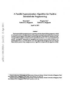
We have performed a set of experiments on a SGI Origin 3800 using up to 32 processors. For our input data we have used complete graphs with random weights on the edges as well as sparse graphs from the University of Florida sparse matrix collection [3]. The top chart of Figure 1 displays the running time for a complete graph on 5000 vertices with random edge weights, as different numbers of processors are applied. As one can see, the running time decreases evenly as more processors are applied. The only exception that is observed is when going from one to two processors, where the running time increases by about 50%. This is due to the extra overhead incurred by the algorithm. In the bottom chart of Figure 1, one can see the running time for the graph crankseg 1 from the University of Florida sparse matrix collection [3]. This is a
3.5
3
2.5
Time
2
1.5
1
0.5
0
0
5
10
15
20
25
30
35
Number of processors 0.9
0.8
Metis Block
0.7
Time
0.6
0.5
0.4
0.3
0.2
0.1
0
0
5
10
15
20
25
30
35
Number of processors
Fig. 1. Running time in seconds for a complete graph with 5000 vertices (top) and for a sparse graph with about 50000 vertices and 5 million edges (bottom).
sparse graph of 52,804 vertices and 5,280,703 edges. For this graph we display both the running time when the graph is partitioned using Metis and when using a block partitioning. As one can observe, there is a significant effect when partitioning the graph using Metis. This is due to much fewer crossing edges when using Metis than when using block partitioning. As a consequence, the algorithm also requires fewer rounds with Metis.
5
Conclusion
In this work, we have shown that the distributed matching algorithm by Hoepman [8] lends itself well to execution on a parallel computer. Moreover, we have shown that this algorithm is closely related to Luby’s maximal independent set algorithm. In the future, we intend to report more detailed results from our experiments including incorporations of our code in existing linear solvers. We will also look more closely at extending the algorithm by using short augmenting paths to improve the approximation ratio of the matching even further.
References 1. D. Avis, A survey of heuristics for the weighted matching problem, Networks, 13 (1983), pp. 475–493. 2. R. H. Bisseling, Parallel Scientific Computation: A Structured Approach Using BSP and MPI, Oxford University Press, 2004. 3. T. Davis, University of Florida sparse matrix collection. http://www.cise.ufl.edu/research/sparse/matrices, NA Digest, vol. 92, no. 42, October 16, 1994, NA Digest, vol. 96, no. 28, July 23, 1996, and NA Digest, vol. 97, no. 23, June 7, 1997. 4. D. E. Drake and S. Hougardy, A linear-time approximation algorithm for weighted matchings in graphs, ACM Transactions on Algorithms, 1 (2005), pp. 107– 122. 5. I. S. Duff and J. Koster, The design and use of algorithms for permuting large entries to the diagonal of sparse matrices, SIAM J. Matrix Anal. Appl., 20 (1999), pp. 889–901. 6. , On algorithms for permuting large entries to the diagonal of a sparse matrix, SIAM J. Matrix Anal. Appl., 22 (2001), pp. 973–996. 7. A. Grama, A. Gupta, G. Karypis, and V. Kumar, Introduction to Parallel Computing, 2nd ed., Addison-Wesley, 2003. 8. J.-H. Hoepman, Simple distributed weighted matchings, arXiv:cs/0410047v1 (2004). 9. G. Karypis and V. Kumar, Metis, a software package for partitioning unstructured graphs, partitioning meshes, and computing fill-reducing orderings of sparse matrices. Version 4.0, 1998. 10. M. Luby, A simple parallel algorithm for the maximal independent set problem, SIAM J. Comput., 15 (1986), pp. 1036–1053. 11. S. Pettie and P. Sanders, A simpler linear time 2/3 − ǫ approximation for maximum weight matching, Inf. Process. Lett., 91 (2004), pp. 271–276. 12. R. Preis, Linear time 1/2-approximation algorithm for maximum weighted matching in general graphs, in Proceedings of STACS ’99, vol. 1563, Lecture Notes in Computer Science, Springer, 1999, pp. 259–269.