A Parallel Implementation of Multi-domain High-order Navier-Stokes

A Parallel Implementation of Multi-domain High-order Navier-Stokes Equations Using MPI Hui Wang1 , Yi Pan2 , Minyi Guo1 , Anu G. Bourgeois2 , Da-Ming Wei1 1 School of Computer Science and Engineering, University of Aizu, Aizu-Wakamatsu, Fukushima 965-8580, Japan {hwang,minyi,dm-wei}@u-aizu.ac.jp Department of Computer Science, Georgia State University, Atlanta, GA 30303, USA {pan,anu}@cs.gsu.edu 2

Abstract In this paper, Message Passing Interface (MPI) techniques are used to implement highorder full 3-D Navier-Stokes equations in multi-domain applications. A two-domain interface with five-point overlap used previously is expanded to a multi-domain computation. There are normally two approaches for this expansion. One is to break up the domain into two parts through domain decomposition (say, one overlap), then use MPI directives to further break up each domain into n parts. Another is to break the domain up into 2n parts with 2n − 1 overlaps. In our present effort, the latter approach is used and finite-size overlaps are employed to exchange data between adjacent multi-dimensional sub-domains. It is general enough to parallelize the high-order full 3-D Navier-Stokes equations into multi-domain applications without adding much complexity. Results with high-order boundary treatments show consistency among multi-domain calculations and single-domain results. These experiments provide new ways of parallelizing 3-D Navier-Stokes equations efficiently.

1

Introduction

Mathematicians and physicists believe that the phenomenon of the waves following boats and the turbulent air currents following flights can be explained through an understanding of solutions to the Euler Equations or Navier-Stokes equations. In fact, Euler Equations are simplified NavierStokes equations. The Navier-Stokes equations describe the motion of a fluid in two or three dimensions. These equations need to be solved for an unknown velocity vector (say, u(x, t)) and pressure vector (say, p(x, t)) with position x and time t. In nonlinear fluid dynamics, the full Navier-Stokes equations are written in strong conservation form for a general time-dependent curvilinear coordinate transformation (x, y, z) to (ξ, η, ζ) [1, 2]: ˆ ˆ ∂ U ∂ Fˆ ∂ G ∂H 1 ∂ Fˆv ∂ Gˆv ∂ Hˆv S ( )+ + + = [ + + ]+ (1) ∂t J ∂ξ ∂η ∂ζ Re ∂ξ ∂η ∂ζ J where F, G, H are inviscid fluxes, and Fv , Gv , Hv are the viscous fluxes. Here, the unknown velocity U = {ρ, ρu, ρv, ρw, ρEt } is the solution vector, and the transformation Jacobian J is a function of time for dynamic meshes. S is the components of a given, externally applied force. 1

Table 1: The parameters, points, and orders for different schemes in common use. Scheme Compact 6 Compact 4 Explicit 4 Explicit 2

Point and Order 5-point, 6th-order 3-point, 4th-order 3-point, 4th-order 1-point, 2nd-order

Γ 1/3 1/4 0 0

a 14/9 3/2 4/3 1

b 1/9 0 -1/3 0

Curvilinear coordinates are defined as those with a diagonal metric so that general metric has gµν ≡ δνµ (hµ )2 with the Kronecker Delta δνµ . Equation (1) is simply Newton’s law f = ma for a fluid element subject to the external force source term S. Until now however, no one has been able to find the full solutions without help from numerical computations since they were originally written down in the 19th Century. In order to discretize the above equations, a finite-difference scheme is introduced [2, 3, 4, 5] because of its relative ease of formal extension to higher-order accuracy. The spatial derivative for any scalar quantity φ, such as a metric, flux component, or flow variable, is obtained in the transformed plane by solving the tridiagonal system: �

�

�

Γφi−1 + φi + Γφi+1 = b

φi+2 − φi−2 φi+1 − φi−1 +a 4 2

(2)

where Γ, a and b determine the spatial properties of the algorithm. Table 1 lists the values of parameters Γ, a and b, points, and orders in common use for different schemes. The dispersion characteristics and truncation error of the above schemes can be found in Reference [2]. A high-order implicit filtering technique is introduced in order to avoid the instabilities, while maintaining the high accuracy of the spatial compact discretization. Filtered values φ¯ satisfy, αf φ¯i−1 + φ¯i + αf φ¯i+1 =

N � an

n=0

2

(φi+n + φi−n )

(3)

where the parameter αf has −0.5 < αf < 0.5. Pade-series and Fourier-series analysis are employed to derive the coefficients a0 , a1 , . . . , aN . Using curvilinear coordinates, up to 10thorder filter formulas has been developed to solve Naiver-Stokes equations. Reference [2] provides a numerical computation method to solve the Navier-Stokes equations. To yield highly accurate solutions to the equations, Visbal and Gaitonde use higher-order finitedifference formulas with emphasis on Pade-type operators, which are usually superior to Taylor Expansions when the functions contain poles, and a family of single-parameter filters. By developing higher-order one-sided filters, Reference [2, 5] obtain enhanced accuracy without any impact on stability. With non-trivial boundary conditions, highly curvilinear three dimensional meshes, and non-linear governing equations, the formulas are suitable in practical situations. Higher-order computation, however, may increase the calculation time. To satisfy the need for highly accurate numerical schemes without increasing the calculation time, parallel computing techniques constitute an important component of modern computational strategy. Using parallel programming methods on parallel computers, we gain access to 2

greater memory and CPU resources not available on serial computers, and are able to solve large problems more quickly. A two-domain interface has been introduced in Reference [5] to solve the Navier-Stokes equations. Suppose there is a two-domain interface, each domain runs first with its input data. While each domain writes and sends the data which are needed by another domain to a temporary file located on hard disk, it also checks and reads the temporary file to retrieve the data output from another domain. This manually treatment, however, has some shortcomings. It requires much more time because it needs to write the data to hard disk. Because of its lowspeed computation and limitation of memory, it is obvious that this method is not convenient to be employed for multi-domain calculations. In our work, parallelizing techniques using Message Passing Interface (MPI) [6, 8, 7, 9] are used to implement high-order full three dimensions Navier-Stokes equations in multi-domain applications on a multiprocessor parallel system. The two-domain interface used in [5] will be expanded to multi-domain computations using MPI techniques. There are two approaches for this expansion. One approach is to break up the domain into two parts through domain decomposition (say, one overlap), then use MPI directives to further break up each domain into n parts. Another approach is to break it up into 2n domains with 2n - 1 overlaps. The later approach is used in this paper and we employ finite-sized overlaps to exchange data between adjacent multi-dimensional sub-domains. Without adding much complexity, it is general enough to treat curvilinear mesh interfaces. Results show that multi-domain calculations reproduce the single-domain results with high-order boundary treatments.

2

Parallelization with MPI

Historically, there have been two main approaches to writing parallel programs. One is to use of a directives-based data-parallel language, and another is to explicit message passing via library calls from standard programming languages. The later approach, such as Message Passing Interface (MPI), is left up to the programmer to explicitly divide data and work across the processors and then manage the communications among them. This approach is very flexible. In our program, there are two different sets of input files with two domains. One data set is xdvc2d1.dat and xdvc2d1.in, and another is xdvc2d2.dat and xdvc2d2.in, respectively. xdvc2d1.dat and xdvc2d2.dat are parameter files, while xdvc2d1.in and xdvc2d1.in are initialized as input metrics files. The original input subroutine DATIN is copied to two input subroutines DATIN1 and DATIN2. All processes are sharing data from one of the input files: IF ( MYID .LT. NPES / 2 ) THEN CALL DATIN1 ELSE IF ( MYID .GE. NPES / 2 ) THEN CALL DATIN2 ENDIF For convenience, the size of the input metrics for each processor is the same for those sharing the same input files. IF ( MYID .LT. NPES / 2 ) THEN IMPI = ILDMY / ( NPES / 2 ) * MYID ELSE IMPI = ILDMY / ( NPES - NPES / 2 ) * ( MYID - NPES / 2 ) ENDIF 3

Mesh 1

1

IL-5

IL-4

2

3

IL-3

IL-2

Mesh 1

Mesh 2

5-pt overlap

4

5

IL-1

Mesh 2

6

IL

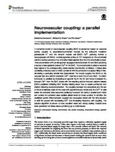
Arrows show information transfer

Figure 1: Schematic of mesh overlap with 5-points in a two-domain calculation [5] ILDMY is the value of size read from input file. In the following codes, ILDMY gets back the value of size for each processor. IF ( MYID .EQ. NPES / 2 - 1 ) THEN ILDMY = ILDMY - ILDMY / ( NPES / 2 ) * ( NPES / 2 - 1 ) ELSE IF ( MYID .EQ. NPES - 1 ) THEN ILDMY = ILDMY - ILDMY / ( NPES - NPES / 2 ) * ( NPES - NPES / 2 - 1) ELSE IF ( MYID .LT. NPES / 2 ) THEN ILDMY = ILDMY / ( NPES / 2 ) ELSE ILDMY = ILDMY / ( NPES - NPES / 2 ) ENDIF All of the above modifications are done in the main program. However, the important part is in subroutine BNDRY, where we add subroutine BNDRYMPI instead of subroutine BNDRYXD in order to process multi-domain computations using MPI techniques. 4

In BNDRYMPI, the communication between different processes are completed by the functions of sending messages and receiving messages. IF ( MYID .GT. 0 ) THEN CALL MPI_SEND, SENDS MESSAGES TO PROCESSOR (MYID - 1) CALL MPI_IRECV, RECEIVES MESSAGES FROM PROCESSOR (MYID - 1) CALL MPI_WAIT ( REQUEST, STATUS, IERR) ENDIF IF (MYID .LT. NPES-1) THEN CALL MPI_SEND, SENDS MESSAGES TO PROCESSOR (MYID + 1) CALL MPI_IRECV, RECEIVES MESSAGES FROM PROCESSOR (MYID + 1) CALL MPI_WAIT ( REQUEST, STATUS, IERR) ENDIF The above calls allocate a communication request object and associate it with the request handle (the argument REQUEST). The request can be used later to query the status of the communication or wait for its completion. Here only nonblocking message communication is used. A nonblocking send call indicates that the system may start copying data out of the send buffer. The sender should not access any part of the send buffer after a nonblocking send operation is called, until the send completes. A nonblocking receive call indicates that the system may start writing data into the receive buffer. The receiver should not access any part of the receive buffer after a nonblocking receive operation is called, until the receive completes. We can see the configuration of these communication in next section.

3

Multi-domain calculation

In this section we introduce the configuration for multi-domain computations. The communication between any adjacent domains is conducted through finite-size overlaps. There is an unsteady flow generated by a convecting vortex in left-side domain(s) and a uniform flow in right-side domain(s). Some parameters are set in common use, such as the non-dimensional vortex strength C/(U∞ R) = 0.02, the sizes of domain −6 < X = x/R < 6, −6 < Y = y/R < 6, 136 × 64 uniformly spaced points with a spacing interval �X = �Y = 0.41, and a timing interval �t = 0.005, where R is the nominal vortex radius. The overlap method in Reference [5] is a successful two-domain calculation method. Therefore, we expand this method when developing the MPI Fortran version of the numerical solution of the Navier-Stokes equations. To illustrate data transfer between the domains, details of a five-point vertical overlap is shown in Figure 1. The vortex was initially located at the center of Mesh 1 (1st domain, solid lines). When computing begins, the vortex moves towards Mesh 2 (2nd domain, dashed lines) with increasing time. The vortex will not stop, but pass through the interface and then convect into Mesh 2 after that. The meshes communicate through an overlap region. In Figure 1, for clarity, the overlap points are shown slightly staggered although they are collocated. At every time-step, data is exchanged between domains at the end of each sub-iteration of the implicit scheme, as well as after each application of the filter. Each vertical line is denoted by its i-index. The data in columns IL − 4 and IL − 3 of the 1st domain were sent to columns 1 and 2 of the 2nd domain, and the data in columns 4 and 5 of the 2nd domain were sent to columns IL − 1 and IL of 1st domain. 5

Single-domain on 1 CPU

2-domain on 1st CPU

2-domain on 2nd CPU

IL-4 IL-3

IL-1 IL

multi-domain

1

2

4

5

multi-domain

on (i-1)th

multi-domain

on ith CPU IL-4 IL-3

1

IL-1 IL

2

4

5

on (i+1)th

IL-4 IL-3

IL-1 IL

1

2

4

5

Figure 2: The sketch map of sending and receiving messages among different processes for single-domain, two-domain, and multi-domain computations. 0.015

0.015

SET 34-35 at T=0 on domain 1 SET 34-35 at T=0 on domain 2

0.01

0.01

0.005

0.005

0

0

-0.005

-0.005

-0.01

-0.01

-0.015 -10

-5

0

5

10

15

SET 34-35 at T=6 on domain 1 SET 34-35 at T=6 on domain 2

-0.015 -10

20

0.015

-5

0

5

10

15

20

SET 34-35 at T=12 on domain 1 SET 34-35 at T=12 on domain 2

0.01

0.005

0

-0.005

-0.01

-0.015 -10

-5

0

5

10

15

20

Figure 3: The swirl velocity as a function of x, obtained in a two-domain calculation with periodic end conditions are compared at three instants, T = 0 (upper-left), 6 (upper-right), and 12 (bottom). Different colors were used to separate velocities of set IL = 34 + 35, JL = 34 on different processors. 6

Multi-domain calculations are performed by using exactly the same principle as in singledomain computations. The only difference is that data are exchanged between adjacent domains at the end of each scheme and after each filtering. Expanding the configuration from two-domain to multi-domain, these transformation are taken between each adjacent domains (processors). The computation is started with the vortex located at the center of Mesh i. With increasing time, the vortex convects into Mesh i + 1 after passing through the interface. The meshes communicate through an overlap region. Each mesh has IL number of vertical lines, which are denoted by its i-index, and JL number of horizontal lines. The values at points 1 and 2 of Mesh 2 are equal to the corresponding values at points IL − 4 and IL − 3 of Mesh 1. Similarly, values at points 4 and 5 of Mesh 2 donate to points IL − 1 and IL of Mesh 1. The exchange of information is shown with arrows at each point in the schematic. Note that although points on line IL − 2 (Mesh 1) and 3 (Mesh 2) are also overlapped, they do not need to communicate directly. This only occurs when the number of overlap points is odd (say, 5 here) and it is called the non-communicating overlap (N CO) point. Figure 2 shows the sketch of sending and receiving messages among different processes in our program. A vertical interface is introduced into the curvelinear mesh as shown schematically.

800

8

Set: IL=136x2,JL=64 Set: IL=68x2,JL=34 Set: IL=34+35,JL=34

700

7

6

500

5

Speedup

Running Time (s)

600

400

300

4

3 200 2

Set: IL=136x2,JL=64 Set: IL=68x2,JL=34 Set: IL=34+35,JL=34

100 1 0 0

2

4

6

8

0

10

2

4

6

8

10

Number of Processors

Number of Processors

Figure 4: Running time and speedup for the set IL = 34 + 35, JL = 34, the set IL = 136 × 2, JL = 64, and the set IL = 68 × 2, JL = 64 versus the number of processors. The number of each line overlap points can be larger and smaller, but there must be at least two points. Reference [5] investigated some odd number of overlap points, specifically 3, 5, 7 points, and the effect of overlap size. By increasing the overlapping size, the instabilities will also increase, and the vortex will be diffused and distorted. In a 3-point overlap, each domain receives data only at an end point, which is not filtered. With larger overlaps, every domain needs to exchange several near-boundary points, that need to be filtered due to the characteristic of the Pade-type formulas. However, filtering the received data can actually introduce instabilities at domain interfaces. On the other side, results show that the accuracy may increase with a 7

larger overlapping region. The 7-point overlap calculation, as opposed to the 3-point overlap calculation can reproduce the single-domain calculation. To keep a balance, schemes with a 5-point horizontal overlap give good performance of reproducing the results of the single domain calculation while keeping the vortex in its original shape. set 136-64 at 2400 with 5 CPUs 0.015

0.01

0.01

0.005

0.005 swirl velocity

swirl velocity

set 136-64 at 2400 with 2 CPUs 0.015

0

0

-0.005

-0.005

-0.01

-0.01

-0.015 -10

-5

0

5 x

10

15

-0.015 -10

20

-5

0.015

0.01

0.01

0.005

0.005

0

-0.005

-0.01

-0.01

-5

0

5

10

10

15

20

15

20

0

-0.005

-0.015 -10

5 x

set 136-63 at 2400 with 10 CPUs

0.015

swirl velocity

swirl velocity

set 136-64 at 2400 with 6 CPUs

0

15

20

x

-0.015 -10

-5

0

5

10

x

Figure 5: Swirl velocities of multi-domain calculation for the set with IL = 136 × 2 and JL = 64 at T = 12 are shown as a function of the number of processors. When specification of boundary treatment is important, the precise scheme will be denoted with 5 numbers, abcde where a through e are numbers denoting the order of accuracy of the formulas employed respectively at points 1, 2, {3· · · IL − 2}, IL − 1 and IL respectively. For example, 45654, consists of a sixth-order interior compact formula, which degrades to 5th- and 4th-order accuracy near each boundary. Explicit schemes in this 5 number notation will be prefixed with an E. The curvlinear mesh in this paper is generated with the parameters xmin = ymin = -6, xmax =18, ymax =6, Ax = 1, Ay = 4, nx = ny = 4, and φx = φy = 0. The 34443 scheme with a 5-point overlap is used to generate results.

8

4

Performance

All of the experiments were performed on a 24 R10000 processors SGI Origin 2000 distributedshared memory multiprocessor system. Each processor has a 200MHz CPU with 4 MB of L2 cache and 2 Gbytes of main memory. The system runs IRIX 6.4. � Begin with a theoretical initial condition, the swirl velocity, (u − u∞ )2 + v 2 , obtained in two-domain calculation with periodic end conditions are compared at three instants, T = 0 (shown in upper-left-side figure), 6 (shown in upper-right-side figure) and 12 (shown in bottomside figure), respectively. At time T = 0, the vortex center is located at X = 0 and, as time increases, it convects to the right at a non-dimensional velocity of unity. The two-domain results are clearly demonstrated in Figure 3 which shows the swirl velocity along Y = 0 at T = 12. The discrepancy in peak swirl velocity between the single- and two-domain computations is negligible. The vortex is well-behaved as it moves through the interface. The contour lines are continuous at the non-communicating overlap point. It shows that the two-domain results reproduce the single-domain values quite well. It also indicates that the higher-order interface treatments are stable and recover the single domain solution. The serious problem we first confront is the correctness of our computation. Comparing the two-domain computation with the manual treatment by Reference [5], it is sure that the results reproduced by the MPI parallel code were found to be in excellent agreement with those in Reference [5]. There are not any difference between them. Speedup figures describe the relationship between cluster size and execution time for a parallel program. If a program has run before (maybe on a range of cluster sizes), we can record past execution times and use a speedup model to summarize the historical data and estimate future execution times. Here, the speedup for the IL = 136 × 2 and JL = 64 set versus the number of processors used is shown in Figure 4 for MPI based parallel calculations. From the figure, we can see that the speedup is close to 8 for 10 CPUs. The reason is that, in five-point overlap treatment, the computation on each processor is almost independent while the costs of the communication between the processors can be disregarded. The speedup is a linear function of the number of processors. It shows that our parallel code with MPI has good performance on partition. The single-domain computation with the same conditions is also included in Figure 4. Since two different input files exist, we can not use MPI based parallel code to calculate using only 1 CPU (processor). The problem can be solved later if one input file is needed. On the other side, the limitation of maximum number of processors depends on the size of horizontal points, IL. Suppose we have a set with IL = 34. More than 6 processors may output error messages because each domain must contain at least about 5 points for exchanging with its adjacent domain. Results of multi-domain calculations for the set with IL = 136 × 2 , JL = 64 are shown in Figure 5. In the figure, the swirl velocities at T = 12 are shown as a function of the number of processors. With a different number of processors, the shape of swirl velocities are very close. This shows that our multi-domain calculation on a multiprocessor system is consistent with single domain results.

5

Conclusion

In this paper, multi-domain high-order full 3-D Navier-Stokes equations were studied. MPI was used to treat the multi-domain computation, which is expanded from the two-domain interface used previously. One single-domain is broken into up to 2n domains with 2n - 1 overlaps. Five finite-sized overlaps are employed to exchange data between adjacent multi-dimensional subdomains. It is general enough to parallelize the high-order full 3-D Navier-Stokes equations 9

into multi-domain applications without adding much complexity. Parallel execution results with high-order boundary treatments show strong agreement between multi-domain calculations and the single-domain results. These experiments provide new ways of parallelizing 3-D NavierStokes equations efficiently.

References [1] D. A. Anderson, J. C. Tannehill, and R. H. Pletcher, Computational Fluid Mechanics and Heat Transfer, McGraw-Hill Book Company, 1984. [2] M. R. Visbal and D. V. Gaitonde, High-Order Accurate Methods for Unsteady Vortical Flows on Curvilinear Meshes. AIAA Paper 98-0131, January 1998. [3] S. K. Lele, Compact Finite Difference Schemes with Spectral-like Resolution. Journal of Computational Physics, 103:16-42, 1992. [4] D. V. Gaitonde, J.S. Shang, and J. L. Young, Practical Aspects of High-Order Accurate Finite-Volume Schemes for Electromagnetics. AIAA Paper 97-0363, Jan. 1997. [5] D. V. Gaitonde and M. R. Visbal, Further Decelopment of a Navier-Stokes Solution Procedure Based on Higher-Order Formulas, AIAA 99-0557, 37th AIAA Aerospace Sciences Meeting & Exhibit, Reno, NV, Jan. 1999. [6] W. Gropp, E. Lush, and A. Skjellum, Using MPI Portable Parallel Programming with the Message-Passing Interface, MIT press, Cambridge, Massachusetts, 1994. [7] P. Pacheco, Parallel programming with MPI, Morgan Kaufmann, San Francisco, California, 1997. [8] M. Snir, S.W. Otto, S. Huss-Lederman, D.W. Walker, and J. Dongarra, MPI The Complete Reference, MIT Press, Cambridge, Massachusetts, 1996. [9] B. Wilkinson, and M. Allen, Parallel Programming, Prentice Hall, Upper Saddle River, New Jersey, 1999.

10