many smaller local optimizations to find a minimum (called 2D Leap-Frog). ... This paper presents a parallel implementation of the 2D Leap-Frog algorithm in.
A PARALLEL LEAP-FROG ALGORITHM FOR 3-SOURCE PHOTOMETRIC STEREO Tristan Cameron Ryszard Kozera∗ Amitava Datta The School of Computer Science and Software Engineering The University of Western Australia 35 Stirling Highway Crawley, W. A., 6009, Perth, Australia
Abstract
Existing Photometric Stereo methods provide reasonable surface reconstructions unless the irradiance image is corrupted with noise and effects of digitisation. However, in real world situations the measured image is almost always corrupted, so an efficient method must be formulated to denoise the data. Once noise is added at the level of the images the noisy Photometric Stereo problem with a least squares estimate is transformed into a non-linear discrete optimization problem depending on a large number of parameters. One of the computationally feasible methods of performing this non-linear optimization is to use many smaller local optimizations to find a minimum (called 2D Leap-Frog). However, this process still takes a large amount of time using a single processor, and when realistic image resolutions are used this method becomes impractical. This paper presents a parallel implementation of the 2D Leap-Frog algorithm in order to provide an improvement in the time complexity. While the focus of this research is in the area of shape from shading, the iterative scheme for finding a local optimum for a large number of parameters can also be applied to any optimization problems in Computer Vision. The results presented herein support the hypothesis that a high speed up and high efficiency can be achieved using a parallel method in a distributed shared memory environment.
Keywords:
Photometric Stereo, Shape from Shading, Nonlinear Optimization, Parallel Processing, Noise Rectification.
∗ This
research was supported by an Alexander von Humboldt Foundation.
2
1.
Introduction
Photometric Stereo consists of two independent steps: gradient computation and gradient integration. Existing linear noise removal algorithms [3, 9] work on the assumption that after the first step of gradient computation the Gaussian nature of the noise is preserved, however, this is not the case and the resulting reconstructed surface can be incorrect as shown in [7, 8]. If we assume the Gaussian noise is added to the irradiance images, and not to the vector fields, then we must take the non-linear setting to solve the optimization problem. This depends (as shown in [7, 8]) on a large number of parameters. Since the numerical scheme for solving such an optimisation task involves the calculation of the Hessians (matrix of second derivatives that will have the size (M × M )2 where M is the image resolution) it is computationally expensive. It would also be very computationally expensive to calculate the eigenvalues of such a large matrix. The 2D Leap-Frog Algorithm proposed in [6–8] is an iterative method that is similar to the block-Gauss-Seidel, but is non-linear [6]. The local optimization is broken into a series of smaller optimization problems (consisting of a smaller number of variables, and thus smaller Hessians) that can be solved much more quickly and with a wider variety of methods. This, however, is offset against the need for many small optimizations to converge to the global optimum. This paper proposes a parallel method for the 2D Leap-Frog Algorithm in order to accelerate the denoising and reconstruction step. The experiments run used three light sources and the initial guess consisted of the ideal surface with added Gaussian noise. The finding of a good initial guess is not covered in this paper and this is a different problem that is present in any non-linear optimization problem. Although the focus of this paper is on denoising shape from shading, the 2D Leap-Frog, and therefore the proposed parallel method, can be applied to any non-linear optimization problem in computer vision. The proposed parallel method would therefore be beneficial to many areas involving image processing or non-linear optimization such as medical imaging, synthetic aperture radar, and robot vision [5].
2D Leap-Frog This section will give a simple geometric explanation of the 2D Leap-Frog Algorithm. Readers are referred to [6–8] for a more detailed definition. The 2D Leap-Frog Algorithm simplifies the large scale optimisation problem by blending solutions of small scale problems in order to converge to the maximum-likelihood estimate of the surface. This means that we have a large choice of ready-made algorithms for optimising the small scale problems (in this case the Levenberg-Marquardt method).
3
A Parallel Leap-Frog Algorithm for 3-source Photometric Stereo
2
1
Figure 1.
Shows the pixels optimized by three different overlapping snapshots.
In practice we deal with discrete data, and so we must define the domain of the 2D Leap-Frog Algorithm. Let our domain be Ω of size M × M , where M is a number of pixels. The domain of the subproblems, called snapshots, is given by Ω m , and has size k × k, where k = 4 pixels in this implementation. Let xn be a pixel in our domain. Then, given an initial guess u0 , the 2D Leap-Frog Algorithm moves to the unique maximum-likelihood estimate uopt of u by the following steps. An iteration begins at snapshot Ω 1 , in the bottom-left corner of Ω. From a snapshot Ω m , we obtain Ω m+1 by translating Ω m the horizontal axis, until the right edge of Ω is reached.
k 2
pixels along
The next snapshot is obtained by translating Ω 1 vertically by and then translating Ω m along the horizontal axis as before.
k 2
pixels,
An iteration is complete when the last snapshot optimised is Ω n , or the top-right corner of Ω. Fig. 1 shows the pixels optimised for each snapshot in the 2D Leap-Frog Algorithm. The snapshots are optimised accoring to the cost function of the 2D LeapFrog Algorithm, called the performance index [6–8]. The performance index measures the distance between the images of the computed solution and the noisy input images and can be defined analytically as follows: E(x1 , x2 , . . . , xN ) =
X
Ei (xi1 , . . . , xik ) + Ej (xj1 , . . . , xjk ) ,
(1)
i6=j
where E is defined over Ω, N is large, ik and jk are small, all components of Ei are fixed, all components of Ej are free, and Ei and Ej are defined over a snapshot Ω m . By finding the optimum of Ej we decrease the energy of E
4 (since all components of Ei are fixed). This procedure finds the suboptimal solution of E and in the case when the initial guess is good this solution is a global minimum.
2.
Parallel Implementation
The approach taken uses a root processor to perform the calculations along with the rest of the processors. The topology here is the one dimensional Cartesian network [4]. A Cartesian, or grid topology consists of all the nodes forming a lattice or grid. Each processor communicates only with the processors connected to it, increasing robustness. The topology used is a grid of width one, meaning processors have at most two processors to communicate with, one above, and one below. The root processor deals with all the initialization details and initial communication and final communication, but it will behave in the same way as the other processors during the core of the algorithm. The image and initial guess are split up in the same way between the processors according to a pre-defined scheme. The image is split up into rows between the processors in as even a way as possible by root. Every set of rows must be divisible by 2 because of the size of the sub-squares used to process the image, which is 4 × 4 in this implementation. However, pixels outside the sub-square are also used in the non-linear optimization process as fixed parameters. This essentially means that when processing a sub-square, access to a 6 × 6, 5 × 6, 6 × 5, or 5 × 5 sub-domain of pixels must be available, depending on the boundary conditions. The consequence of this is that once the root processor has defined how the image is to be split among the processors, an ‘overlap’ row is added to the bottom and top of each set of rows. The bottom, or root, processor only receives a top overlap row and the top processor only receives a bottom overlap row. An important feature to note here is that the 2D Leap-Frog Algorithm converges to a globally minimal solution (given a good initial guess) due to the many overlapping local minimizations. This means that if the individual processors are allowed to work entirely independently of each other the convergence would not be guaranteed. This is because the sub-squares that are contained in the top two rows (excluding the overlap row) of processor n and the bottom two rows (excluding the overlap row) of processor n + 1 would never be processed. This area, called the ‘buffer zone’, must be processed prior to each iteration of the 2D Parallel Leap-Frog. Once these buffer zones have been processed, each processor is able to run the 2D Leap-Frog Algorithm on its remaining data. It must be noted that at the end of the processing of the buffers and at the end of each iteration processors must be synchronized for the communication of the buffer data.
A Parallel Leap-Frog Algorithm for 3-source Photometric Stereo
5
Parallel Efficiency The efficiency of a parallel algorithm is expressed in terms of speed up, Sp = T1 /Tp , where T1 is the time taken for one processor to finish the computation, and Tp is the time taken using p processors to finish the computation. The efficiency is given by Ep = Sp /p. It should be noted that in general 1/p ≤ Ep ≤ 1. So far when talking about speed up and efficiency we have been concerned with the computational time only. However, the performance of a distributed memory architecture must also take into account the communication time. The time taken for a program to run on p processors is given by Tp = (T1 /p) + Tc , where T1 is the time taken to run on a single processor and Tc is the communication time of the program. We can now apply this to the formula for speed up above to give us T1 Sp = . (2) (T1 /p) + Tc
Expected Efficiency Using (2) from above, we can calculate an expected speed up, and therefore an expected efficiency of the proposed parallel method. Let Tc = n/To where Tc is the communication time in seconds, n is the number of bytes to send, and To is the number of bytes that can be sent per second. During the initialization phase p − 1 processors receive approximately 4M/p rows (each row consists of M double (8 byte) values). Each processor recieves approximately M/p rows from each of the three irradiance images and from the initial guess. After the 2D Leap-Frog Algorithm has finished processing, p − 1 processors send approximately M/p rows (each row consisting of M double values) to the root processor. During a single iteration of the 2D Parallel Leap-Frog Algorithm using p processors, p − 1 processors send 2 rows each containing M double values at the beginning of the buffer processing. Following the buffer processing p − 1 processors send 2 rows each containing M double values. The number of bytes that can be sent per second, To , is approximately 500,000,000 bytes [1]. This gives us the following equation for the expected communication time:
Tc =
8 ((p − 1)(4M/p) + (p − 1)(M/p)) + (8 ∗ 500(4M (p − 1))) , (3) 500000000
where M is the image resolution and p is the number of processors Note that the number of iterations is fixed at 500. This can be substituted into (2) to give an expected speed up.
6
(a)
(b)
(c)
Figure 2. (a) The ideal surface with a performance index of zero. (b) The initial guess with a performance index of 88.451. (c) The reconstructed surface with a performance of 5.055.
3.
Results
Experiments were carried out on a 4 node AlphaServer SC40 at the Interactive Virtual Environments Center (IVEC) [2] known as CARLIN. Each node consists of four 667 MHz Alpha EV67 processors and has access to 4GB of main memory, with up to 108 GB of virtual memory. Each processor has a 64KB L-cache, 64KB D-cache, and 8 MB of Level 2 cache [2]. The non-linear local minimization technique used was the Levenberg-Marquardt algorithm. The experimental surfaces were tested at three differing resolutions so as to ascertain the scalability of the algorithm. A total of four surfaces were tested however, due to space limitations the reconstructions for only one will be presented in this paper. The timings for all four surfaces will be reported. Two of the surfaces tested were synthetic and two of the surfaces were of real data, one a jug and one a fish, both generated from 3D Studio Max models. The reconstruction of the Jug is shown in the results. The three different image resolutions tested were 64 × 64, 128 × 128, and 256 × 256 pixels. This gives us an idea how the implementation scales from a small image (64 × 64) to a large image (256 × 256). For each experiment noise from a Gaussian (Normal) distribution with mean 0 and standard deviation 0.2 was added to the ideal surface to generate the initial guess. The irradiance images, with intensity values ranging from 0 to 1, were corrupted with noise from a Gaussian distribution with mean 0 and standard deviation 0.02. It is expected that the speed up will be relatively high (efficiency above 60%) for the eight processor implementation.
4.
Conclusion
As can be seen in Fig. 2(c) the reconstructed surface provides a reasonable representation of the ideal surface shown in Fig. 2(a). The value of the perfor-
A Parallel Leap-Frog Algorithm for 3-source Photometric Stereo
7
mance index [7, 7, 8] is also much closer to zero (ideal) for the reconstructed surface than that of the initial guess. From Fig. 3, Fig. 4, and Fig. 5 it can be seen that the speed up was higher for the large resolution images than for the smaller resolution images. This is as expected since, when reconstructing the surface with a higher resolution, a larger percentage of the total time is spent in parallel processing as opposed to communication. The results given support our hypothesis even though the actual speed up is lower than the expected speed up. This is because the expected speed up was calculated using the maximal throughput of 500 MB per second when in reality this would rarely be achieved. Due to the effectiveness of this parallel algorithm, reconstructions can be done in far less time, and with a greater accuracy through more iterations.
References [1] Hewlett-packard company. http://www.hp.com, 2003. Accessed 7/10/2003. [2] Interactive virtual environments centre. http://www.ivec.org, 2003. Accessed 4/9/2003. [3] Robert T. Frankot and Rama Chellappa. A method for enforcing integrability in shape from shading algorithms. IEEE Trans. Pattern Anal. Mach. Intell., 10(4):439–451, 1988. [4] A. Grama, A. Gupta, G. Karypis, and V. Kumar. Introduction to Parallel Computing. Addison Wesley, 2003. [5] B. K. P. Horn. Robot Vision. MIT Press in association with McGraw-Hill, 2001. [6] L. Noakes and R. Kozera. A 2D Leap-Frog algorithm for optimal surface reconstruction. Proc. 44th Annual Meet. Opt. Eng. SPIE’99, III-3811:317–328, 1999. [7] L. Noakes and R. Kozera. Denoising images: Non-linear Leap-Frog for shape and lightsource recovery. Chapter in Theoretical Foundations of Computer Vision Geometry, Morphology and Computational Images, pages 419–436, 2003. Lecture notes in Computer Science 2616. [8] L. Noakes and R. Kozera. Nonlinearities and noise reduction in 3-source photometric stereo. J. Math. Imag. and Vis., 2(18):119–127, 2003. [9] T. Simchony, R. Chellappa, and M. Shao. Direct analytical methods for solving Poisson equations in computer vision problems. IEEE Trans. Pattern Rec. Mach. Intell., 12(5):435– 446, 1990.
8
Time (sec) vs Number of Processors
8
Speed Up
Time (sec)
Expected 1
6
300 250 200
4 3
100
2
2
3
4
5
6
Number of Processors
7
1 1
8
0.2
2
3
4
5
7
0 1
8
Time (sec) vs Number of Processors
8
3
4
5
6
Number of Processors
7
8
(c)
Speed Up vs Number of Processors
Efficiency vs Number of Processors Expected
7
1600
1
6
1200 1000 800
Expected
0.8
Efficiency
Speed Up
1400
5 4
Actual
0.6
0.4
3
Actual
600
0.2
2
400 2
3
4
5
6
Number of Processors
7
1 1
8
2
3
4
5
6
Number of Processors
(a)
7
0 1
8
2
3
4
5
6
Number of Processors
(b)
Figure 4.
7
8
(c)
The results for the 128 by 128 resolution images.
8
Time (sec) vs Number of Processors
Speed Up vs Number of Processors
Efficiency vs Number of Processors Expected
7
10000 9000
1
6
7000 6000 5000
4 3
4000 3000
0.8
Expected
5
Efficiency
Speed Up
8000
Time (sec)
2
The results for the 64 by 64 resolution images.
1800
11000
6
Number of Processors
(b)
Figure 3.
200 1
Actual 0.6
0.4
Actual
(a)
Time (sec)
0.8
Expected
5
150
2000
Efficiency vs Number of Processors
7
350
50 1
Speed Up vs Number of Processors
Efficiency
400
Actual 0.6
0.4
Actual
0.2
2
2000 1000 1
2
3
4
5
6
Number of Processors
(a)
Figure 5.
7
8
1 1
2
3
4
5
6
Number of Processors
(b)
7
8
0 1
2
3
4
5
6
Number of Processors
(c)
The results for the 256 by 256 resolution images.
7
8