Journal of Reliability and Statistical Studies; ISSN (Print): 0974-8024, (Online):2229-5666 Vol. 7, Issue 1 (2014): 103-112
A PARALLEL SYSTEM WITH ARRIVAL TIME OF EXPERT SERVER SUBJECT TO MAXIMUM REPAIR AND INSPECTION TIMES OF ORDINARY SERVER S.C. Malik1 and Gitanjali2 Department of Statistics, M.D. University, Rohtak-124001 (India) 2 Department of Mathematics, NIEC, GGSIPU, Delhi (India) E Mail:
[email protected],
[email protected]
1
Received December 24, 2013 Modified June 02, 2014 Accepted June 05, 2014 Abstract A parallel system of two identical units has been analyzed stochastically considering two types of servers. Initially, the unit is repaired by the ordinary sever who visits the system immediately. And, when ordinary server is unable to do repair of that unit in a given maximum repair time, the unit undergoes for inspection to see the feasibility of its repair by an expert server. If inspection reveals that repair of the unit is also not possible by the expert server, then it is replaced by new unit. The expert server takes some time to arrive at the system. The failure rate of each unit and rate by which unit undergoes for inspection by the ordinary server are taken as constant while the distributions of arrival, inspection, repair and replacement times are assumed as arbitrary with different probability density functions. All random variables are statistically independent. The expressions for several reliability measures are derived using semi-Markov process and regenerative point technique. Graphs are drawn to depict the behavior of MTSF, availability and profit for different values of the parameters.
Key Words: Parallel System, Two Servers, Maximum Repair Time and Reliability Measures. 2000 Mathematics Subject Classification: 90B25 and 60K10
Introduction Method of redundancy has widely been used in many industrial plants to increase their reliability and safety. Nakagawa (1980) and Singh (1989) analyzed the systems with cold standby redundancy under different sets of assumptions on failure and repair policies. But there exist many systems in which cold standby redundancy is not suggestive and so it is desirable to introduce parallel redundancy. For example, in a power supply system, the transformers having same polarity and voltage ratio are connected in parallel in order to meet the total load requirements as well as to provide continuous power supply for essential services. Kishan and Kumar (2009) and Kumar et al. (2010) investigated stochastic models of parallel systems by taking single server for rectification of faults. But sometimes complex faults may occur in the system during operation which cannot be repaired by an ordinary server in a given time. In that situation an expert server may be called to get the repair done. Otherwise, the unit may be replaced by new one in order to avoid the unnecessary expenses on repair. Malik and Gitanjali [2012] discussed a parallel system with arrival and maximum repair times of ordinary server.
104
Journal of Reliability and Statistical Studies, June 2014, Vol. 7(1)
In view of the above observations and facts, the aim of the present paper is to determine reliability measures of a parallel system of two identical units with repair by two servers – one is ordinary and the other is an expert. Initially, the unit is repaired by the ordinary sever who visits the system immediately. The ordinary server inspects the unit after a maximum repair time to see the feasibility of its repair by an expert server. When inspection reveals that repair of the unit is not also possible by the expert server then it is replaced with new by the ordinary server. The expert server takes some time to arrive at the system. The failure rate of unit and rate by which unit undergoes for inspection are taken as constant while the distributions of arrival time of the expert server, inspection time, repair time and replacement time of the unit are assumed as arbitrary with different probability density functions. All random variables are statistically independent. The switch over is instantaneous and perfect. The unit works as new after repair. The expressions for several reliability measures of vital significance are derived using semi-Markov process and regenerative point technique. The numerical results pertaining to the particular case have been obtained to depict the graphical behavior of MTSF, availability and profit with respect to the replacement rate.
Notations 𝐸 𝑂 𝜆 𝛼0
: : : :
a/b
:
𝑡 /𝐻 𝑡
:
𝑓 𝑡 /𝐹 𝑡
:
𝑤e (𝑡)/𝑊e 𝑡 𝑔 𝑡 /𝐺 𝑡
:
𝑔1 𝑡 /𝐺1 𝑡
:
𝐹𝑈𝑟 / 𝐹𝑈𝑅
:
𝐹𝑊𝑟 / 𝐹𝑊𝑅
:
𝐹𝑊𝑟𝑒 / 𝐹𝑊𝑅𝑒
:
𝐹𝑈𝑖 / 𝐹𝑈𝐼
:
Set of regenerative states. Unit is operative. Constant failure rate of the unit. Constant rate by which unit under goes for inspection after a pre-specified time ‘t’ to see the feasibility of repair. Probability that failed unit is not repairable / repairable by an expert server. pdf/cdf of the inspection time of the unit taken by ordinary server. pdf/cdf of the replacement time of the unit taken by ordinary server. pdf / cdf of the waiting time of the expert server for repairing of the failed unit. pdf / cdf of the repair time of the unit taken by ordinary server. pdf / cdf of the repair time of the unit taken by expert server. Unit is failed and under repair / under repair continuously from previous state. Unit is failed and waiting for repair by ordinary server / waiting for repair by ordinary server continuously from previous state. Unit is failed and waiting for repair by expert server / waiting for repair by expert server continuously from previous state. Unit is failed and under inspection with ordinary server / waiting for inspection by ordinary server continuously from previous state.
105
A Parallel System with Arrival Time of Expert Server...
𝐹𝑈𝑟𝑒 /𝐹𝑈𝑅𝑒
:
𝐹𝑈𝑟𝑝 / 𝐹𝑈𝑅𝑃
:
𝑚𝑖𝑗
:
𝜇𝑖
:
~/∗
:
𝑺 /©
:
Unit is failed and under repair with expert server / under repair continuously from previous state with expert server. Unit is failed and under replacement / under replacement continuously from previous state. Contribution to mean sojourn time in state 𝑆𝑖 ∈ 𝐸 and non-regenerative state if occurs before transition to 𝑆𝑗 ∈ 𝐸. Mathematically, it can be written as ∞ ′ 𝑚𝑖𝑗 = 0 𝑡 𝑑 𝑄𝑖𝑗 𝑡 = −𝑞𝑖𝑗 ∗ 0 . The mean sojourn time in state 𝑆𝑖 which is given by ∞ 𝜇𝑖 = 𝐸 𝑇 = 0 𝑃 𝑇 > 𝑡 𝑑𝑡 = 𝑗 𝑚𝑖𝑗 , where 𝑇 denotes the time to system failure. Symbol for Laplace Stieltjes transform / Laplace transform. Symbols for Stieltjes convolution / Laplace convolution.
The possible transitions between states along with transitions rates for the system model are shown in figure 1.The states 𝑆0 , 𝑆1 , 𝑆2 , 𝑆3 , 𝑆4 and 𝑆5 are regenerative while the other states are non-regenerative.
Transition Probabilities and Mean Sojourn Times Simple probabilistic considerations yield the following expressions for the non-zero elements 𝑝𝑖𝑗 = 𝑄𝑖𝑗 ∞ = 𝑞𝑖𝑗 𝑡 𝑑𝑡 as 𝛼0 𝑝01 = 1 , 𝑝10 = 𝑔 ∗ 𝜆 + 𝛼0 , 𝑝12 = 𝛼 +𝜆 1 − 𝑔 ∗ 𝜆 + 𝛼0 , 𝑝17 = 𝛼
𝜆
0 +𝜆
0
1 − 𝑔 ∗ 𝜆 + 𝛼0 ,
𝑝23 = 𝑎∗ 𝜆 , 𝑝24 = 𝑏∗ 𝜆 , 𝑝2,11 = 1 − ∗ 𝜆 ,
𝑝30 = 𝑓 ∗ 𝜆 , 𝑝36 = 1 − 𝑓 ∗ 𝜆 , 𝑝45 = 𝑤𝑒 ∗ 𝜆 , 𝑝50 = 𝑔1 ∗ 𝜆 , 𝑝5,14 = (1 − 𝑔1 ∗ 𝜆 ), 𝑝61 = 𝑓 ∗ 0 , ∗ 𝑝78 = 1 − 𝑔 𝛼0 , 𝑝89 = 𝑎, 𝑝8,10 = 𝑏, 𝑝91 = 𝑓 ∗ 0 𝑝11,9 = 𝑎, 𝑝11,10 = 𝑏, 𝑝12,1 = 𝑔1 ∗ 0 , 𝜆 𝑝14,1 = 𝑔1 ∗ 0 , 𝑝11.7 = 𝛼 +𝜆 1 − 𝑔 ∗ 𝜆 + 𝛼0 𝑔 ∗ 𝛼0 , 𝑝11.7,8,9 = 𝛼
𝑎𝜆 0
0
[1-g*(λ+𝛼0)](1-𝑔 ∗ 𝛼0 ), +𝜆
𝑝11.7,8,10,12 = 𝛼
𝑏𝜆
0 +𝜆
𝑝4,13 = 1 − 𝑤𝑒 ∗ 𝜆 𝑝71 = 𝑔 ∗ 𝛼0 𝑝10,12 = 𝑤𝑒 ∗ 0 𝑝13,12 = 𝑤𝑒 ∗ 0
, , , ,
[1-g*(λ+𝛼0)](1-𝑔 ∗ 𝛼0 ),
𝑝21.11,9 = 𝑎 1 − ∗ 𝜆 , 𝑝21.11,10,12 = 𝑏 1 − ∗ 𝜆 , 𝑝31.6 = 1 − 𝑓 ∗ 𝜆 , ∗ ∗ 𝑝41.13,12 = 1 − 𝑤𝑒 𝜆 , 𝑝51.14 = 1 − 𝑔1 𝜆 1 It can easily be verified that 𝑝01 = 𝑝10 + 𝑝12 + 𝑝17 = 𝑝10 + 𝑝12 + 𝑝11.7 + 𝑝11.7,8,9 + 𝑝11.7,8,10,12 = 𝑝23 + 𝑝24 + 𝑝2,11 = 𝑝23 + 𝑝24 + 𝑝21.11,9 + 𝑝21.11,10,12 = 𝑝30 + 𝑝36 = 𝑝30 + 𝑝31.6 = 𝑝45 + 𝑝41.13,12 = 𝑝45 + 𝑝4,13 = 𝑝50 + 𝑝5,14 = 𝑝50 + 𝑝51.14 = 𝑝61 = 𝑝71 + 𝑝78 = 𝑝89 + 𝑝8,10 = 𝑝91 = 𝑝10,12 = 𝑝11,9 + 𝑝11,10 = 𝑝12,1 = 𝑝13,12 = 𝑝14,1 = 1 2 The mean sojourn times 𝜇𝑖 in state 𝑆𝑖 is given by ∞ 1 1 𝜇0 = 0 𝑃 𝑇 > 𝑡 𝑑𝑡 = m01 = 2λ, 𝜇1 = m10 + m12 + m17 = 𝛼 +𝜆 1 −
𝑔∗𝜆+𝛼0,
𝜇2=m23+m24+m2,11=1𝜆1−∗𝜆,
0
106
Journal of Reliability and Statistical Studies, June 2014, Vol. 7(1) 1
𝜇3 = m30 + m36 = 𝜆 1 − 𝑓 ∗ 𝜆
1
𝜇4 = m45 + m4,13 = 𝜆 1 − 𝑤𝑒 ∗ 𝜆 ,
,
1
𝜇5 = m50 + m5,14 = 𝜆 1 − 𝑔1 ∗ 𝜆 , 𝜇1′ = m10 + m12 + m11.7 + m11.7,8,9 𝑔 ∗ 𝛼0
1 α0
+ m11.7,8,10,12
=
1−g ∗ α0 +λ α0 +λ
[1 + λ 1 −
− 𝑏𝑔1 ∗ ′ 0 − 𝑎𝑓 ∗ ′ 0 − ∗ ′ 0 − b𝑤𝑒 ∗ ′ 0 ]
𝜇2′ = m23 + m24 + m21.11,9 + m21.11,10,12 = 1 − ∗ 𝜆 𝑎𝑓 ∗ ′ 0 + ∗ ′ 0 + b𝑤𝑒 ∗ ′ 0
1 𝜆
− 𝑏𝑔1 ∗ ′ 0 +
, 1
𝜇3′ = m30 + m31.6 = 1 − 𝑓 ∗ 𝜆
𝜆
− 𝑓∗ ′ 0 ,
𝜇4′ = m45 + m41.13,12 = 1 − 𝑤𝑒 ∗ 𝜆
=
𝜇5′ = m50 + m51.1.4 = 1 − 𝑔1 ∗ 𝜆
1 𝜆
1 𝜆
− 𝑔1 ∗ ′ 0 + 𝑤𝑒 ∗ ′ (0) ,
− 𝑔1 ∗ ′ 0 .
3
Mean Time to System Failure (MTSF)
Let φi t be the cdf of first passage time from the regenerative state to a failed state 𝑆𝑖 . Regarding the failed state as absorbing state, we have the following recursive relations for φi t : φi t = j Qi,j t S φj t + k Qi,j t (4) where Sj is an un-failed regenerative state to which the given regenerative state Si can transit and k is a failed state to which the state i can transit directly. Taking LST of above relation (4) and solving for 𝝋0 𝑠 , we get 1−φ 𝑠 𝑁 𝑀𝑆𝑇𝐹 𝑇0 = lim𝑠→0 𝑠0 = 𝐷1 (5) 1
Where 𝑁1 = 𝜇0 + 𝜇1 + 𝑝12 𝜇2 + 𝑝12 𝑝23 (𝜇3 + 𝑝24 𝜇4 + 𝑝24 𝑝45 𝜇5 ) and 𝐷1 = 1 − 𝑝10 − 𝑝12 𝑝23 𝑝30 + 𝑝24 𝑝45 𝑝5,14 .
Availability Analysis Let Ai (t) be the probability that the system is in up-state at instant 't' given that the system entered regenerative state Si at t = 0. The recursive relations for Ai (t) are given as (𝑛) Ai t = 𝑀𝑖 𝑡 + j 𝑞𝑖,𝑗 t © 𝐴𝑗 𝑡 (6) where Mi(t) is the probability that the system is up initially in regenerative state Si ∈ 𝐸 at time ′𝑡` without visiting to any other regenerative state and 𝑀0 𝑡 = 𝑒 −2𝜆𝑡 , 𝑀1 𝑡 = 𝑒 − 𝜆 +α 0 𝑡 𝐺 𝑡 , 𝑀2 𝑡 = 𝑒 −𝜆𝑡 𝑡 𝐻 𝑡 , −𝜆𝑡 −𝜆𝑡 𝑀3 𝑡 = 𝑒 𝑡 𝐹 𝑡 𝑀4 𝑡 = 𝑒 𝑡 𝑊𝑒 𝑡 , 𝑎𝑛𝑑 𝑀5 𝑡 = 𝑒 −𝜆𝑡 𝑡 𝐺1 𝑡 ∗ Taking 𝐿. 𝑇. of relation 6 and solving for 𝐴0 𝑠 , we get steady-state availability as 𝑁 A0(s) =limA0*(s) =𝐷 2 (7) 𝑠→0
2
Where 𝑁2 = 𝑝10 + 𝑝12 𝑝23 𝑝30 + 𝑝24 𝑝45 𝑝50 𝜇0 + 𝜇1 + 𝑝12 𝜇2 + 𝑝12 (𝑝23 𝜇3 + 𝑝24 𝜇4 + 𝑝24 𝑝45 𝜇5 ) and 𝐷2 = 𝑝10 + 𝑝12 𝑝23 𝑝30 + 𝑝24 𝑝45 𝑝50 𝜇0 + 𝜇1′ + 𝑝12 𝜇2′ + 𝑝12 (𝑝23 𝜇3′ + 𝑝24 𝜇4 ′ + 𝑝24 𝑝45 𝜇5 ′).
A Parallel System with Arrival Time of Expert Server...
107
Busy Period Analysis of Ordinary Server Due to Repair
Let 𝐵𝑖𝑅 𝑡 be the probability that the ordinary server is busy in repairing the unit at an instant ‘𝑡’given that the system entered regenerative state Si at 𝑡 = 0. The recursive relations for 𝐵𝑖𝑅 𝑡 are given as (n) BiR t = Wi t + j qi,j t © BjR t (8) where 𝑊1 𝑡 = 𝑒 − 𝜆 +𝛼 0 𝑡 𝐺 𝑡 + 𝜆𝑒 −𝜆𝑡 ©𝟏©𝑒−𝛼 0 𝑡 𝐺 𝑡 (9) 𝑅∗ Taking 𝐿. 𝑇. of relation 8 and solving for𝐵0 𝑠 , we get in the long run the time for which the system is under repair is given by 𝑁 ∗ 𝐵0𝑅 = lim𝑠→0 𝑠 𝐵0𝑅 𝑠 = 𝐷3 (10) 2
Where 𝑁3 = 𝑊1∗ 0 and 𝐷2 is already specified.
Busy Period Analysis of Ordinary Server Due To Replacement 𝑅𝑝
Let 𝐵𝑖 𝑡 be the probability that the ordinary server is busy in repairing the unit at an instant ‘𝑡’given that the system entered regenerative state Si at 𝑡 = 0.The 𝑅𝑝 recursive relations for 𝐵𝑖 𝑡 are given as Rp (n) Rp Bi t = Wi t + j qi,j t © Bj t (11) −𝜆𝑡 −𝜆𝑡 Where 𝑊3 𝑡 = 𝑒 𝐹 𝑡 + 𝜆𝑒 ©𝟏© 𝐹 𝑡 (12) 𝑅𝑝 ∗
Taking 𝐿. 𝑇. of relation 11 and solving for 𝐵0 𝑠 , we get in the long run the time for which the system is under replacement is given by 𝑁 𝑅𝑝 𝑅𝑝 ∗ 𝐵0 = lim𝑠→0 𝑠 𝐵0 𝑠 = 𝐷4 (13) 2
where 𝑁4 = 𝑝12 𝑝23 𝑊3∗ 0 and 𝐷2 is already specified.
Busy Period Analysis of Ordinary Server Due To Inspection
Let 𝐵𝑖𝑖 𝑡 be the probability that the ordinary server is busy in inspection of the unit at an instant ‘𝑡’given that the system entered regenerative state Si at 𝑡 = 0. The recursive relations for 𝐵𝑖𝑖 𝑡 are given as (n) Bi𝑖 t = Wi t + j qi,j t © Bji t (14) Where 𝑊2 𝑡 = 𝑒 −𝜆𝑡 𝐻 𝑡 + 𝜆𝑒 −𝜆𝑡 ©𝟏 𝐻 𝑡 15 𝑖∗ Taking 𝐿. 𝑇. of relation 14 and solving for𝐵0 𝑠 , we get in the long run the time for which the system is under inspection is given by ∗ 𝑁 𝐵0𝑖 = lim𝑠→0 𝑠 𝐵0𝑖 𝑠 = 𝐷5 16 2
Where 𝑁5 = 𝑝12 𝑊2∗ 0 and 𝐷2 is already specified.
Busy Period Analysis of Expert Server Due To Repair
Let 𝐵𝑖𝑒 𝑡 be the probability that the expert sever is busy in repairing the unit at an instant ‘ 𝑡 ’given that the system entered regenerative state Si at 𝑡 = 0. The recursive relation for 𝐵𝑖𝑒 𝑡 are given by: (n) Bi𝑒 t = Wi t + j qi,j t © Bje t (17) Where 𝑊5 𝑡 = 𝑒 −𝜆𝑡 𝐺1 𝑡 + 𝜆𝑒 −𝜆𝑡 ©𝟏 𝐺1 𝑡 18 Taking 𝐿. 𝑇. of relation 17 and solving for 𝐵0𝑒∗ 𝑠 , we get the time for which the system is under repair done by expert server is given by 𝑁 𝐵0𝑒 = lim𝑠→0 𝑠 𝐵0𝑒∗ 𝑠 = 𝐷6 19 2
108
Journal of Reliability and Statistical Studies, June 2014, Vol. 7(1)
where 𝑁6 = 𝑝12 𝑝24 𝑝45 𝑊5∗ 0 and 𝐷2 is already specified.
Expected Number of Visits by the Ordinary Server
Let 𝑁𝑖 𝑡 be the expected number of visits by the ordinary server in 0, 𝑡 given that the system entered the regenerative state Si at 𝑡 = 0 . The recursive relation for 𝑁𝑖 𝑡 are given by (𝑛) 𝑁𝑖 𝑡 = 𝑗 𝑄𝑖,𝑗 𝑡 𝑆 𝛿𝑗 + 𝑁𝑖 𝑡 (20) Where δj =1, if Sj is the regenerative state where the ordinary server does job afresh, otherwise δj = 0. Taking 𝐿. 𝑆. 𝑇. of relation 20 and solving for 𝑁0 𝑠 , we get the expected number of visits by ordinary server per unit time as 𝑁 𝑁0 = lim𝑠→0 𝑠 𝑁0 𝑠 = 𝐷7 (21) 2
Where
𝑁7 = 𝑝10 + 𝑝12 𝑝23 𝑝30 + 𝑝24 𝑝45 𝑝50
and 𝐷2 is already specified.
Expected Number of Visits by Expert Server
Let 𝑁𝑖𝑒 𝑡 be the expected number of visits by expert server 0, 𝑡 given that the system entered the regenerative state Si at 𝑡 = 0. The recursive relation for 𝑁𝑖𝑒 𝑡 are given by: (𝑛 ) 𝑁𝑖𝑒 𝑡 = 𝑗 𝑄𝑖,𝑗 𝑡 𝑆 𝛿𝑗 + 𝑁𝑖𝑒 𝑡 (22) Where δj =1, if Sj is the regenerative state where the expert server does job afresh, otherwise δj = 0. Taking 𝐿. 𝑆. 𝑇. of relation 22 and solving for 𝑁0𝑒 𝑠 , we get the expected number of visits by expert server per unit time as 𝑁 𝑁0𝑒 = lim𝑠→0 𝑠 𝑁0𝑒 (𝑠) = 𝐷8 23 2
Where 𝑁8 = 𝑝12 𝑝24 + 𝑝11.7,8,10,12 + 𝑝12 𝑝21.11,10,12
and
𝐷2 is already specified.
Expected Number of Replacements of the Unit
Let 𝑅𝑖 𝑡 be the expected number of replacement of unit in 0, 𝑡 given that the system entered the regenerative state Si at 𝑡 = 0 . The recursive relation for 𝑅𝑖 𝑡 are given by (𝑛) 𝑅𝑖 𝑡 = 𝑗 𝑄𝑖,𝑗 𝑡 𝑆 𝛿𝑗 + 𝑅𝑖 𝑡 (24) 𝛿𝑗 =1, if Sj is the regenerative state where the ordinary server does job afresh, otherwise 𝛿𝑗 = 0. Taking 𝐿. 𝑆. 𝑇. of relation 24 and solving for 𝑅0 𝑠 , we get the expected number of replacements per unit time as 𝑁9 𝑅0 = lim 𝑠 𝑅0 𝑠 = 25 𝑠→0 𝐷2 Where N9=𝑝12 𝑝23 + 𝑝11.7,8,9 + 𝑝12 𝑝21.11,9 and 𝐷2 is already specified.
Cost-Benefit Analysis Profit incurred to the system model in steady state is given 𝑅𝑝 𝑃 = 𝐾1 𝐴0 − 𝐾2 𝐵0𝑅 − 𝐾3 𝐵0 − 𝐾4 𝑅0 −𝐾5 𝐵0𝑖 − 𝐾6 𝐵0𝑒 − 𝐾7 𝑁0 − 𝐾8 𝑁0𝑒 Where 𝐾1 = Revenue per unit uptime of the system
by
A Parallel System with Arrival Time of Expert Server...
𝐾2 𝐾3 𝐾4 𝐾5 𝐾6 𝐾7 𝐾8
= = = = = = =
109
Cost per unit time for which ordinary server is busy due to repair Cost per unit time for which ordinary server is busy due to replacement Cost per unit time replacement of the unit Cost per unit time for which ordinary server is busy due to inspection Cost per unit time for which expert server is busy due to repair Cost per unit visits by the ordinary server Cost per unit visits by the expert server
Conclusion To make the study more concrete and informative, numerical results for the particular case 𝑡 = 𝜃𝑒 −𝜃𝑡 , 𝑔1 𝑡 = 𝜃0 𝑒 −𝜃0 𝑡 , 𝑓 𝑡 = 𝛽𝑒 −𝛽𝑡 , 𝑤 𝑡 = 𝛾𝑒 −𝛾𝑡 , 𝑤𝑒 𝑡 = 𝛾0 𝑒 −𝛾0 𝑡 and 𝑡 = 𝜂𝑒 −𝜂𝑡 are obtained to depict the graphical behavior of MTSF, availability and profit function with respect to replacement rate (β) keeping fixed values of other parameters including 𝐾1 = 5000, 𝐾2 = 600, 𝐾3 = 100, 𝐾4 = 450, 𝐾5 = 50, 𝐾6 = 900, 𝐾7 = 150, 𝐾8 = 200 with 𝑎 = 0.6 and 𝑏 = 0.4 as shown in figures 2 to 4 respectively. It is observed that MTSF, availability and profit of the system model go on increasing with the increase of replacement rate (β), repair rate (θ) of ordinary server, repair rate (θ0) of expert server, inspection rate (η) of the unit and arrival rate (γ0) of the expert server while their values decrease as the rate (𝞪0) by which unit undergoes for inspection and failure rate (λ) increases. Furthermore, system becomes less profitable for K2 < K4. Thus, a parallel system of two identical units in which expert server takes some arrival time at the completion of maximum repair time of the ordinary server can be made more profitable to use by increasing the repair rate of ordinary server in case replacement cost is high.
References 1.
2.
3.
4. 5.
Kishan, R. and Kumar, M. (2009). Stochastic analysis of a two-unit parallel system with preventive maintenance, Journal of Reliability and Statistical Studies. 2(2), p. 31-38. Kumar, J., Kadyan, M.S. and Malik, S.C. (2010). Cost- benefit analysis of a two-unit parallel system subject to degradation after repair, Applied Mathematical Sciences. 4(56), p. 2749-2758. Malik, S.C. and Gitanjali (2012). Cost-Benefit Analysis of a Parallel System with Arrival Time of the Server and Maximum Repair Time, International Journal of Computer Applications, 46 (5), p. 39-44. Nakagawa, T. (1980). Optimum inspection policies for a standby unit, J. Oper. Res. Soc., Japan., 23, p. 13-27. Singh, S.K. (1989). Profit evaluation of a two-unit cold standby system with random appearance and disappearance time of the service facility, Microelectronics and Reliability. 29, p. 705-709.
Acknowledgement The authors are grateful to the reviewers for giving suggestions which enable us to improve the worth of the paper.
110
Journal of Reliability and Statistical Studies, June 2014, Vol. 7(1)
State Transition Diagram 𝑆0
g(t)
o
𝑆8
𝑆1
𝑆7 λ
o
o
𝐹𝑈𝑟
2λ 𝑆6
f(t)
𝑆3 o
α0
ah(t)
ah(t)
𝑆5 o
𝑆10 𝑆11
o
𝐹𝑊𝑟
λ
𝐹𝑊𝑅
𝐹𝑈𝐼
𝐹𝑈𝑖
bh(t)
𝐹𝑊𝑟𝑒
𝑆12
𝑆14 λ
bh(t)
𝐹𝑈𝑅𝑝
𝑆2
𝐹𝑈𝑅𝑝 𝑔1 (t)
ah(t)
𝐹𝑊𝑅
𝑔1 (t)
𝑔1 (t)
λ
𝐹𝑈𝑖
𝑆9 f(t)
𝐹𝑈𝑅𝑃
𝐹𝑊𝑅
𝐹𝑈𝑅
g(t)
F𝑊𝑟
f(t)
α0
F𝑊𝑟
𝐹𝑈𝑅𝑒
𝐹𝑊𝑅
bh(t)
𝐹𝑊𝑟
𝐹𝑈𝑟𝑒 𝑆13
𝑆4 o
𝑤𝑒 (t)
𝐹𝑊𝑟𝑒
𝐹𝑈𝑟𝑒
O
: : :
λ
𝐹𝑊𝑟 𝐹𝑊𝑅𝑒
Regenerative Point Upstate Failed State Figure. 1
𝑤𝑒 (t)
𝑤𝑒 (t)
A Parallel System with Arrival Time of Expert Server...
Figure 2
Figure 3
111
112
Journal of Reliability and Statistical Studies, June 2014, Vol. 7(1)
Figure 4