... and Econometricians, in particular Ãyvind Eitrheim, Andreas Fischer, Hans .... widespread use among analysts of monetary policy (see for example Blix, 1995, ...
A Parametric Approach for Estimating Core Inflation and Interpreting the Inflation Process*
Mikael Apel, Per Jansson Sveriges Riksbank, S-103 37 Stockholm, Sweden
April 1999
Abstract In this paper we propose a new parametric approach for measuring core inflation and analysing the inflation process. In the model, measured inflation may change because of changes in three basic factors: long-run conditions, transitory output, and ”special factors”. The “special factors” include supply shocks and other factors that affect inflation over and above changes in long-run conditions and transitory output. None of the three basic factors can be directly observed, but each factor is econometrically identified. We show that our approach can be used to derive estimates of core inflation that parallel three different views found in the literature -- as long-run inflation, demanddriven inflation, and inflation excluding certain undesired “special factors”. The approach is illustrated using Swedish quarterly data covering the time period 1970:1-1998:1. Key Words: Core inflation, Kalman filter, structural time-series models, underlying inflation, unobserved-components models. JEL Classification System Numbers: C32, E31.
* We are grateful for useful comments from colleagues at the central bank of Norway and from seminar participants at Sveriges Riksbank and the 1999 BIS meeting of Central Bank Model Builders and Econometricians, in particular Øyvind Eitrheim, Andreas Fischer, Hans Lindblad, and Anders Vredin. The views in this paper are those of the authors and do not necessarily reflect those of Sveriges Riksbank.
1
2
1. Introduction In the last decade, inflation targeting has become a widely used framework for both theoretical analysis and practical design of monetary policy.1 In this framework, the primary objective of the central bank is to keep inflation in line with the target, mainly by affecting real economic activity through appropriate adjustments of its instrument rate. This task may seem straightforward but is in practice associated with considerable difficulties. One problem pertains to the identification and selection of an appropriate target variable. The common view of inflation-targeting central banks seems to be that not all movements in the general price level are equally important from a monetary policy point of view. For example, if an increase or decrease in inflation is perceived to be sufficiently temporary, a policy response may not be regarded as necessary. This suggests that central banks wish to avoid basing their monetary-policy decisions on inflation changes that are not part of the “pure” inflationary process, and rather focus on the underlying, or core, rate of inflation.2 Unfortunately, underlying inflation is a variable that cannot be directly observed.3 Another problem is related to the determination of the component of real economic activity that the central bank can affect through its policy. According to the widely accepted notion of long-run neutrality of money, the central bank can affect real economic activity only temporarily. However, like underlying inflation, the transitory component of output that can be affected by monetary policy is not observable. An interpretation of the task of the central bank is therefore that it has to control an unobservable variable – underlying inflation – mainly through the effects of interest rates on another unobservable variable – a transitory component of output. This is obviously a rather intricate task. Somewhat surprisingly, and adding to the complexity of the problem, the concept of core inflation appears to have no clear theoretical definition. As indicated above, it is usually interpreted as some more persistent component of measured inflation, but different approaches seem to refer to different parts of persistent inflation. In the literature, it is possible to identify at least three different views on core inflation. The first, proposed by Eckstein (1981), interprets core inflation as “the rate [of inflation] that would occur on the economy’s long-term growth path, provided the path were free of shocks, and the state of demand were neutral in the sense that markets were in long-run equilibrium”. (Eckstein, 1981, p. 8.) In what follows we label this view on core inflation “long-run inflation”, reflecting the fact that it in this view is seen as a steady-state concept.4 A second view, introduced by Quah & Vahey (1995), looks at core inflation as “that component of measured inflation that has no (medium- to) long-run impact on [real] output”. (Quah & Vahey, 1995, p. 1130.) An alternative way of putting this is as that component of inflation that is generated by shocks with no (medium- to) long-run effects on real output. Because shocks with no long-run effects on real output are often referred to as demand shocks (Blanchard & Quah, 1989), the Quah-Vahey view on core inflation may alternatively be interpreted as approximately corresponding to the demanddriven component of inflation. A third view, which in what follows is referred to as the “central-bank view”, seeks to capture core inflation by eliminating or reducing the influence of certain factors, typically particularly volatile and erratic components (see for example Blinder, 1982a). Since demand shocks are not in general considered to be among these “undesirable” components, this view on core inflation differs from that of Eckstein, in which the state of demand, as noted above, is required to be neutral at the core rate of inflation.5 It also seems to differ from the Quah-Vahey interpretation since not only demand shocks are assumed to matter for core inflation.
1
Surveys are given in, for example, Leiderman & Svensson (1995), Haldane (1995, 1997), Debelle (1997), and Mishkin & Posen (1997). In this paper, the terms core inflation and underlying inflation are used synonymously. 3 In this context it is however important to note that the policy implications from targeting the core or headline rate of inflation not necessarily need to be different. An inflation-targeting central bank usually bases its actions on a forecast of inflation. Only to the extent that the forecast of headline inflation differs from the forecast of core inflation will the policy actions then differ. This will happen if there are foreseeable effects, for example temporary effects, which affect the forecast of headline inflation but not the forecast of core inflation. The difference between the policy actions is hence likely to depend on the central bank’s target horizon. 4 Scadding (1979) suggested a similar interpretation. 5 See Blinder (1982b). 2
3
In this paper we propose a new parametric approach for measuring core inflation and interpreting the inflation process. The approach takes the unobservability of both core inflation and its determinants explicitly into consideration and estimates these unobservable components simultaneously. In the model, measured inflation may change because of changes in three basic factors: long-run conditions, transitory output, and “special factors”. The “special factors” include supply shocks and other factors that affect inflation over and above changes in long-run conditions and transitory output. None of the three basic factors can be directly observed, but each factor is econometrically identified and thus possible to estimate. Our approach has several interesting features. Firstly, because it explicitly identifies the determinants of inflation within a theoretical model, it allows a decomposition of inflation into economically interpretable components. This facilitates the understanding and analysis of the inflation process. Secondly, and as a corollary of the above-mentioned aspect, we are able to derive estimates of core inflation that parallel the above-discussed different views on this variable. A measure closely related to Eckstein’s (1981) approach is obtained by letting core inflation correspond to the part of inflation generated by long-run conditions, that is when the influences of transitory output and “special factors” are eliminated. Given that transitory output is assumed to reflect the state of aggregate demand, which is the common interpretation in this type of model, a measure corresponding to Quah & Vahey’s (1995) approach is obtained by letting the part of inflation generated by transitory output represent core inflation. The central-bank measure, finally, is obtained by merely excluding the effects of certain of the “special factors” from the measured inflation rate. Thirdly, because our approach is parametric, different specifications of the processes of the determinants of inflation (and hence also of core inflation) may be considered. This may help us to improve our understanding of the inflation process in Sweden (which is the country that we study), but it also may make the approach usable for applications to other countries. The remainder of the paper is structured as follows. Section 2 gives a brief review of the approaches to estimating core inflation that can be found in the literature. Section 3 presents our parametric model of the inflation process and discusses how it relates to the above-mentioned views on core inflation. The empirical illustrations are presented and discussed in Section 4. Section 5, finally, provides concluding remarks.
2. Different Views on Core Inflation 2.1. Long-Run Inflation According to the framework in Eckstein (1981), inflation can be divided into three components: core inflation, a component related to aggregate demand, and a “shock” component. Core inflation is interpreted as the inflation rate that would occur on the economy’s long-term growth path in the absence of shocks and at a neutral state of demand – that is, as the inflation rate that would occur in long-run equilibrium; long-run inflation for short.6 Eckstein develops an econometric model of the US economy, which he uses to decompose actual inflation into these three components. Parkin (1984) shows that this concept of core inflation essentially coincides with the expected rate of inflation in a traditional expectations-augmented Phillips (or aggregate supply) curve.7 Despite the fact that an immense number of Phillips curves have been estimated in different contexts, Phillips-curve specifications have rarely been used to explicitly estimate core inflation interpreted in this way. A possible explanation is that this steady-state interpretation of core inflation seems to be rarely used outside (and possibly also inside) the academic sphere and is probably not what people in general have in mind when referring to the term.
6
This long-run interpretation of the core-inflation concept can also be found in macroeconomic textbooks. See, for example, Burda & Wyplosz (1993) and Romer (1996). 7 See also Scadding (1979, p. 8) who argues that core (underlying) inflation “presumably comes close to the theoretical notion of the perceived rate of inflation”.
4
2.2. The Quah-Vahey Approach An alternative approach for estimating core inflation was introduced by Quah & Vahey (1995). Like the Eckstein framework, this approach establishes a link between core inflation and other economic variables. Core inflation is seen as the component of measured inflation that has no (medium- to) longrun impact on real output. This restriction is in Quah & Vahey (1995) implemented in a bivariate output-inflation vector-autoregressive (VAR) system by assuming that there exist (permanent) shocks that do not affect real output in the long run. These shocks are then assumed to be the shocks that generate core inflation. In the literature, shocks with no long-run impact on output have often been interpreted as demand shocks. Thus, in the Quah-Vahey framework, core inflation may be interpreted as demand-driven inflation (although Quah & Vahey themselves do not explicitly make this interpretation). This view of core inflation seems to differ from other views on the concept. Looking at core inflation as the component of measured inflation that has no (medium- to) long-run impact on real output implies that core inflation is associated with transitory movements of real output out of longrun equilibrium. This contrasts with the interpretation of Eckstein, who assumes that core inflation is the rate of inflation that would occur when the real economy is at its long-run equilibrium. The view also differs from the central-bank view, which does not assume that core inflation only depends on demand shocks. Although no central bank to our knowledge is currently using an estimate derived from the Quah-Vahey approach as its official estimate of underlying inflation, the approach has certainly gained widespread use among analysts of monetary policy (see for example Blix, 1995, Fase & Folkertsma, 1997, Bjørnland, 1997, Claus, 1997, Dewachter & Lustig, 1997, and Gartner & Wehinger, 1998). 2.3. The Central-Bank View The approaches for estimating core inflation emanating from the central-bank view may be loosely described as various ways of eliminating or reducing different “undesirable” effects on the measured inflation rate. Typically, measured inflation is adjusted for highly volatile components and price developments considered to be representing one-off shifts in the price level, such as changes in indirect taxes. Sometimes, measured inflation is also adjusted with respect to the direct, more or less definitional, adverse effects of the central bank’s own actions. In many countries, components directly related to interest-rate changes are left out of the inflation measure since, for example, a tightening of monetary policy will through these components increase measured inflation autonomously. Clearly, such an adverse short-term effect is hardly an adequate reason for further monetary tightening.8 A common feature of the practical implementations of the central-bank approaches is that they, unlike the approaches of Eckstein (1981) and Quah & Vahey (1995), do not establish an explicit link between core inflation and other economic variables. Hence, they tend to have a weaker theoretical under-pinning and may therefore be viewed as more “mechanical”. On the other hand, they are less complicated and thus easier for the general public to understand, at least in the sense that the operations made to arrive at the core-inflation estimate are quite straightforward. Data on the different aggregate price index components (in practice, CPI components) are often used as the starting point for the analysis of core inflation according to the central-bank view. One commonly used approach attempts to make measured inflation reflect the underlying rate more accurately by removing the estimated effects of specific disturbances and events on a case-by-case basis.9 The most common example of this type of correction is adjustment for the effects of changes in indirect taxes. Other events that sometimes are believed to motivate an adjustment are significant changes in the terms of trade or different types of natural disasters causing large price increases on certain items.10 This procedure requires adequate information regarding the source, magnitude, and timing of the disturbance on the price series concerned, which may often be difficult to obtain. 8
See, for example, Roger (1994). See, for example, Roger (1994) and Ravnkilde Erichsen & van Riet (1995). The escape clauses of the institutional monetary-policy framework of New Zealand (see for example Mishkin & Posen, 1997, p. 38) may be viewed as a type of (implicit) case-by-case adjustment in that they allow the central bank to temporarily disregard certain inflation impulses and to accommodate first-round effects on prices, but not to allow the passing on of these effects to a second round. 9
10
5
Adjustment is primarily made with respect to the first-round effects, which may be less uncertain than the successive feed-through effects of the shocks. In the case of indirect-tax adjustments, first-round effects are often calculated by simply using the change in the tax rate and the weight in the CPI of the items in question. However, even first-round effects may be difficult to determine since they may vary over time, for example due to varying opportunities for firms to absorb price shocks in the profit margins, and it may be unclear exactly which items that are affected. Furthermore, a seemingly temporary price shock may affect inflation expectations and thereby feed through into the more persistent parts of inflation. Hence, case-by-case adjustment necessarily contains a judgmental ad-hoc element and may, as a result, sometimes be viewed as a less transparent method. Another frequently used approach intended to make measured inflation correspond more closely to underlying inflation is the so-called excluding-food-and-energy approach which implies that certain price series are completely removed from the aggregate price index. For example, the inflation rate relevant for monetary-policy decisions in the US excludes changes in food and energy prices while the inflation-target variable in the UK is adjusted for mortgage interest payments. Contrary to the case-bycase approach, adjustments are made systematically according to a pre-specified rule and they may therefore be regarded as more transparent.11 A disadvantage of the excluding-food-and-energy approach is that it requires an ex ante identification of the price series to be excluded, which may not always be an easy task. This is illustrated by the finding in Cecchetti (1997) that the CPI excluding food and energy is, in fact, not less volatile than the CPI itself. Furthermore, one can hardly be certain that the excluded price series never contain information on core inflation. Changes in excluded price series may for example at some point in time and under certain circumstances affect inflation expectations and hence feed into the more persistent parts of inflation in the same way as some of the disturbances eliminated in the case-by-case approach. It is also possible that the composition of the group of items whose price behaviour differs from the behaviour of prices in general changes over time. The once-and-for-all choice of the items to be excluded therefore runs the risk of generating an estimate of underlying inflation that over time becomes misleading. The basic idea in the case-by-case and excluding-food-and-energy approaches is that because the overall price index is calculated as a weighted mean of the prices of individual items, the importance of temporary disturbances will be overstated. This is also the point of departure for an approach using so-called limited-influence estimators (LIEs) to analyse core inflation. One type of LIE, suggested by Bryan & Pike (1991), is the weighted median across the number of individual prices.12 The median will differ from the mean when the distribution of individual price changes is skewed. This may be the case when, for example, a period of poor weather raises the price of certain items temporarily. The skewed distribution generates a transitory increase in the mean whereas the median may not be affected (or, at least, less affected). Bryan & Cecchetti (1994) provide a theoretical justification for the use of LIEs, based on the framework in Ball & Mankiw (1995). In the absence of shocks, Bryan & Cecchetti assume that firms raise their prices in line with underlying inflation. When a relative price shock (or cost shock) occurs, the firms affected have to decide whether or not to change their prices at a rate differing from the underlying rate. Changing the price is assumed to be associated with an adjustment cost (menu cost), which implies that the shocks have to be sufficiently large to trigger such a price change. If the cost is large enough, then the firms will choose not to react to the shock and we would as a result find a spike in the cross-sectional price-change distribution at the rate of inflation representing core inflation. Furthermore, above and below certain cut-off points determined by the adjustment costs we would find a lower and an upper tail representing firms hit by shocks large enough to induce deviating price changes despite the adjustment costs. If the distribution of the underlying shocks is, for example, skewed to the right, we would in the distribution of realised price changes expect to find an upper tail that is larger than the lower tail. The most common inflation measure – the mean of realised price changes -- would be influenced by both the spike and the tails and would hence over-estimate core inflation. The median, on the other hand, would only regard the spike, which, according to the assumptions, represents core inflation. 11 It should be noted that the excluding-food-and-energy approach is often used as a complement to the case-by-case approach. It is for example common to adjust for changes in indirect taxes and at the same time exclude certain volatile price series. 12 The weighted median is obtained by ordering the individual items in the aggregate index with respect to the magnitude of the price change, accumulating the weights and picking the price increase of the item corresponding to an accumulated weight of half of the total weight.
6
An advantage of the weighted median compared to the case-by-case and excluding-food-andenergy approaches is that it is completely systematic in the sense that no arbitrary judgement concerning what shocks to adjust for or what price series to disregard from is needed. Furthermore, Bryan & Cecchetti (1994) conclude that among a number of different estimates of core inflation, the weighted median performs best in many respects, for example regarding the ability of the estimate to forecast future price changes. Another LIE is the trimmed mean, suggested by, for example, Bryan & Cecchetti (1994). This estimator is computed by trimming a percentage from the tails of the distribution of individual price changes, and averaging what is left. Thus, the weighted median may be seen as a special case of the trimmed mean where 50 percent has been removed from each tail of the distribution of price changes. Bryan, Cecchetti & Wiggins (1997) and Cecchetti (1997) investigate the efficiency properties of different estimators on US data. They find that the mean with around 10 percent trimmed from each tail is the most efficient estimator of core inflation.13 The choice of how much to trim from the tails is however not obvious. Shortcomings that the LIEs share with the above-discussed other central-bank estimates are that it is difficult to give the estimates an explicit economic content (for example, how they relate to changes in demand and supply) and that there is a risk of excluding potentially important information. 3. A Parametric Model of the Inflation Process As mentioned above, the approach that we propose is based on the idea that the link between inflation and other economic variables can be summarised in a model where inflation is a function of three basic factors: long-run conditions, transitory real output, and “special factors”.14 The approach may be regarded as an application of the so-called structural time-series or unobserved-components (STM/UC) methodology.15 In this section we present the model and discuss some of its properties and implications. Let π t be the measured (CPI) inflation rate, π tLR long-run inflation, ytTRAN the relevant transitory component of real output, Zt a vector of “special factors” (to be defined below) normalised so that E(Zt ) = 0 , and ε t an IID error with zero mean and constant variance σ ε2 . The key equation of our model may then be written as: LR TRAN π t − π tLR = α 1 (π t −1 − π tLR + −1 ) + ... + α p (π t − p − π t − p ) + β 0 y t
β 1 ytTRAN + ... + β q ytTRAN + δ 0Zt + δ 1Zt −1 + ... + δ m Zt −m + ε t , −1 −q or, equivalently,
α ( L)(π t − π tLR ) = β ( L) ytTRAN + δ ( L) Z t + ε t ,
(3.1)
where L is the lag operator, Li xt = xt −i for any variable x. Thus, the short-run component of measured inflation (π t − π tLR ) depends on a transitory component of real output ( ytTRAN ) and a vector of “special factors” (Zt ) , or, equivalently, measured inflation (π t ) depends on long-run inflation (π tLR ) ,
ytTRAN , and Zt . A formal justification of our interpretation of π tLR as the inflation rate that occurs in the long run will be given below. Equation (3.1) bears a rather close resemblance to traditional Phillips (or aggregate supply) curves (see, for example, Gordon, 1997, and Hall & Mankiw, 1994). In some respects, however, the equation differs from traditional Phillips-curve specifications. One difference is that long-run inflation 13
A thirty-six month centred moving average of actual inflation is used as a representation of core inflation. Our framework is hence conceptually similar to that of Eckstein (1981). 15 See, for example, Harvey (1989) for a general reference. Examples of other applications of the STM/UC methodology are Apel & Jansson (1997, 1998) and Gerlach & Smets (1997). 14
7
enters (3.1) as an explicitly identified component which is allowed to vary over time. Usually, the term that we label long-run inflation (which in traditional expectation-augmented Phillips-curve specifications corresponds to expected inflation) is assumed to be constant (captured by the mean rate of inflation) or equal to the inflation rate in the previous period (whereby the change of inflation enters the left-hand side of equation (3.1)). The equation thus allows for a separate identification of the dynamics associated with changes in short-run and long-run inflation (the dynamics of long-run inflation will be discussed below). In a specification with no long-run inflation dynamics (a constant π tLR ), the actual persistence of measured inflation has to originate from one or several of the following sources: (1) the autoregressive lags of measured inflation; (2) the transitory output terms; (3) the “special factors” included in the Zt vector. Equation (3.1) adds to these sources of persistence by allowing for different dynamics of inertia with respect to short- and long-run inflation. In this type of specification, the Zt vector is generally regarded as a vector of supply-shock proxies, intended to capture shifts in the Phillips curve (see, for example, Gordon, 1997).16 Ignoring the influence of supply changes is likely to give rise to mis-specification problems (see Apel & Jansson, 1997, for further discussions of this point). In the present application it will be useful to divide the Zt vector into two sub-categories. The first category (Zt ,1 ) contains the “undesirable” components that the central bank wishes to exclude when making its analysis of core inflation (see the discussion in Section 2.3). The second category ( Z t , 2 ) includes (other) supply-shock proxies that improve the fit of the equation but that here have no direct implications for the estimates of core inflation. From the discussion in the previous section it is clear that the central-bank approach to estimating core inflation in practice involves a substantial judgmental element when it comes to deciding on what disturbances and/or price series to adjust for. Hence, in our implementation of the procedure, there are several possible candidates for variables to include in Zt ,1 . In general, of course, the choice of variables in Zt ,1 (as well as Zt ,2 ) is a non-trivial issue that involves both theoretical and empirical considerations. In our empirical application, we let the procedures and estimates of the Swedish central bank (which are similar to those of other central banks) serve as guidelines when deciding on what variables to include in Zt ,1 , and how they are allowed to enter equation (3.1). In this vector we therefore include data on changes in short-term nominal interest rates, changes in (the log of) nominal oil prices and nominal import prices, and dummies representing changes of indirect taxes. Furthermore, only the contemporaneous effects of these variables are considered. The Zt ,2 vector contains changes in (the log of) labour productivity and relative oil prices.17 Equation (3.1) can then be re-written as:
α( L )( π t − π tLR ) = β ( L ) ytTRAN + δ 0,1Zt ,1 + δ 2 ( L )Zt ,2 + ε t , where δ 0 ,1 captures the contemporaneous impact of the variables in Zt ,1 and δ 2 ( L ) =
(3.2) m
∑δ i =0
i ,2
Li .
Although the problem of selecting appropriate Zt variables is present also in this parametric approach, some interesting differences compared to many of the previously discussed methods can be identified. To elaborate somewhat on this point, it is useful to rewrite equation (3.2) as:
16
If (3.1) is viewed as an aggregate supply relationship, then
εt
is also usually interpreted as a supply shock.
17
For purposes of identification, it is assumed that changes in real oil prices do not have an immediate impact on measured inflation. Although not problem-free, this assumption does not appear unreasonable in light of the fact that “behavioural” changes presumably show up with some lags. The data are quarterly and run from 1970:1 to 1998:1. For further details, see Appendix 1.
8
π t = π tLR + α ( L) −1 β ( L) ytTRAN + α ( L) −1δ 0,1Z t ,1 + α( L ) −1 δ 2 ( L )Zt ,2 + α( L ) −1 ε t .18
(3.3)
Firstly, because we measure the variables’ effects on inflation econometrically rather than using the weights of the items in the CPI, we may, at least to some extent, be able to capture the interdependence between different items. For example, an increase in the price of oil may give rise to contemporaneous price increases in a large number of items in the CPI basket. By estimating the average impact of changes in the price of oil (captured in δ 0 ,1 ) rather than just using the weight of oil in the basket, it may be possible to obtain a more accurate measure of these effects on overall CPI inflation. Secondly, the fact that the specification contains dynamics of short-run inflation implies that it is possible to take into account potential dynamic feed-through effects of changes in the Zt ,1 variables (as well as, of course, of changes in Zt ,2 and ytTRAN ). These effects are in this model reflected in the α( L ) −1 term. For example, a change in an indirect tax may, due to inflation inertia, have effects in several consecutive periods. Just considering the first-round effect, possibly by simply using the change in the tax rate and the weight in the CPI of the items hit by the tax, may therefore give misleading results.19 In Phillips-type equations it is common to interpret the transitory component of output, ytTRAN , as an estimate of the “output gap”. Since changes in aggregate demand are frequently regarded as the main source of business-cycle fluctuations, the output gap (or the unemployment gap) is often regarded as a measure of excess demand. The state of demand may hence be considered to be neutral when ytTRAN = 0 . In most empirical studies, the transitory part of output (or unemployment) is calculated separately and inserted as an exogenous variable in the Phillips-curve specification. In the present STM/UC approach, however, it is possible to treat the transitory part of output as an endogenous variable and estimate it simultaneously with long-run inflation and the parameters of the model. In the preceding section, three different views on core inflation were described. Equation (3.3) can be used to illustrate these views. In long-run equilibrium at a neutral state of demand and in the absence of shocks, equation (3.3) implies that π = π LR .20 This provides a justification for our interpretation of π tLR as the rate of inflation that occurs in the long run. A core inflation estimate closely related to the one proposed by Eckstein (1981) then obtains as:
π tCORE = π tLR .21
18
In going from (3.2) to (3.3) it is assumed that the polynomial
(3.4)
α(L )
is invertible so that short-run inflation,
π t − π tLR , does not contain
any unit roots. 19
Such dynamic feed-through effects could also have been allowed for by including lags of the variables in
Z t ,1 . However, at a conceptual
level, we find it in our case more natural to model these as arising because of inflation inertia. More generally then, one may wish to consider different sets of AR parameters associated with short-run inflation changes depending on the source of the change of inflation. Because our empirical applications are foremost meant as illustrations we have chosen not to address this issue further, but we note that it is an interesting generalisation (although presumably not problem-free from a technical point of view) to be considered in future applications. 20
The precise statement is:
y tTRAN = Z t ,1 = Z t , 2 = ε t = 0 for all t ⇒ π = π LR provided α(1) ≠ 0 .
21 It deserves here to be noted that the measurement of core inflation according to a strict interpretation of Eckstein’s approach cannot be dealt with without knowing the precise nature of the sources of time variation that are prevalent in the process of long-run inflation. For example, if long-run inflation is driven by some stochastic shocks, then core inflation needs to be measured conditionally on the effects of these shocks (in order to fulfil the “in-absence-of-shocks” criterion). In our applications, we shall generally allow the estimates of core inflation interpreted as corresponding to the Eckstein view to depend on stochastic shocks, but it is emphasised that the estimates corresponding to the stricter interpretation obtain as simple special cases in which restrictions on certain parameters are imposed (that is, zero restrictions on the variances of long-run inflation). If all the sources of time variation are regarded as ultimately originating from shocks, then, intuitively, the Eckstein approach to core inflation has to predict that core inflation always is constant. In (3.3) then, core inflation is equal to the constant unconditional expectation of actual inflation. But, in this case, of course, there is no “estimation prob lem”.
9
In the framework of Quah & Vahey (1995), core inflation is basically interpreted as the demand-driven component of inflation. In our model, this would correspond to the second term of the right-hand side of equation (3.3):
π tCORE = α( L ) −1 β ( L ) ytTRAN . 22
(3.5)
The central-bank view, in which the influence of different “undesirable” effects on measured inflation is reduced or eliminated, is in this framework most naturally approximated by subtracting the contemporaneous term δ 0,1 Z t ,1 from measured inflation. Hence, core inflation according to the central-bank view is taken to be:
π tCORE = π t − δ 0,1Zt ,1 = π tLR + α( L ) −1 β ( L ) ytTRAN + (α( L ) −1 − 1) δ 0,1Zt ,1 + α( L ) −1 δ 2Zt ,2 + α( L ) −1 ε t .
(3.6a)
An advantage of our parametric approach, which is clear from the second equality in equation (3.6a), is that the resulting central-bank estimate of core inflation, in contrast to more mechanically derived estimates in this tradition, can be decomposed into economically interpretable components. As discussed previously, it is within this approach also possible to derive a “dynamically adjusted” central-bank estimate of core inflation:
π tCORE = π t − α( L ) −1 δ 0,1Zt ,1 = π tLR + α( L ) −1 β ( L ) ytTRAN + α( L ) −1 δ 2Zt ,2 + α( L ) −1 ε t .
(3.6b)
Thus, the quantity (α ( L) −1 − 1)δ 0,1 Zt ,1 may be regarded as a measure of the importance of the dynamic feed-through effects associated with changes in Zt ,1 . To be able to estimate equation (3.2), it is necessary to specify a parametric process for long-run inflation, π tLR . In STM/UC applications, the most common assumption is that “permanent” unobservable long-run variables follow random walks. In our case this would mean that π tLR is I(1) and satisfies: LR π tLR = π tLR , −1 + ε t
(specification A)
(3.7a)
where ε tLR is an IID error term with E( ε tLR ) = 0 and a constant variance σ ε2LR . However, in the case of Sweden, one may question whether a non-stationary I(1) process like (3.7a) provides a reasonable approximation of the behaviour of long-run inflation during the entire sample period. From the early 1970s until the beginning of the 1990s, recurrent cost crises in Sweden were accommodated by several devaluations (and a depreciation when the fixed exchange rate was abandoned in November 1992). Both the mean and the variance of inflation were high and one may well argue that the Swedish economy during this period lacked a reliable nominal anchor. Shortly after the switch to a floating exchange-rate regime in 1992, an explicit inflation target of 2 percent was introduced. Since then inflation has been low and reasonably stable. 22 It is of course difficult to translate the structural VAR framework of Quah & Vahey to the Phillips-curve framework used in this paper in a fully satisfactory way. One important difference is that the demand-generated part of inflation is assumed to be an I(1) process in Quah & Vahey whereas it in our specification – as equation (3.5) makes clear – is an I(0) variable. We emphasise that the I(1) assumption used by Quah & Vahey is not a necessary condition for applying the Blanchard-Quah identification scheme of demand shocks. If actual inflation instead is assumed to be I(0), then the bivariate VAR system would be driven by a permanent and a purely transitory shock. No further identifying assumptions would be needed to achieve exact identification. A stationary demand-driven component of inflation, consistent with the identification scheme of Blanchard & Quah, could then be computed by setting all permanent shocks equal to zero. This procedure, presumably, would generate a Quah-Vahey core inflation estimate which, at least from an empirical point of view, would be easier to compare with the estimate derived from equation (3.5).
10
Against this background, we consider the following two alternative specifications of the process of π : LR t
π LR + u t ,1 t ≤ 1992 : 4 π tLR = t −1 , µ + u t ,2 t > 1992 : 4
(specification B)
(3.7b)
µ 1 + ηt ,1 t ≤ 1992 : 4 π tLR = , µ 2 + ηt ,2 t > 1992 : 4
(specification C)
(3.7c)
where µ , µ 1 , and µ 2 are constants and u t ,1 , u t ,2 , ηt ,1 , and ηt ,2 innovations that are assumed to be IID with E (u t ,1 ) = E (u t , 2 ) = E (η t ,1 ) = E (η t , 2 ) = 0 and constant variances σ u21 , σ u22 , σ η21 , and σ η22 . Thus, the switch to a regime with an explicit inflation target is assumed to have affected the process for long-run inflation. In specification B, π tLR is assumed to follow a random walk in the period before the switch and to fluctuate randomly around a constant thereafter. In specification C, long-run inflation is assumed to fluctuate randomly around a constant in both periods, but the constants may be different for the two periods. Note that in (3.7c), long-run inflation will be equal to the constant unconditional expectation of actual inflation as µ 1 = µ 2 and σ η2 1 = σ η2 2 = 0 (see footnote 21). It is by no means obvious that the regime shift occurred exactly at the point in time assumed above. Different types of data give a mixed guidance. For example, survey data on inflation expectations of households and agents on the money market show that households started to revise their expectations downwards already before the switch to the floating exchange-rate regime while agents on the money market did not start to revise their expectations downwards until after the switch. Thus, this evidence suggests the possibility of a smooth, rather than discrete, transition to the new regime. However, given the considerable technical difficulties associated with modelling a smooth transition to the new regime, we have in this illustrative application chosen to restrict ourselves to processes that imply a discrete shift. Given this, it seems quite reasonable to let the shift coincide with the switch to the floating exchange-rate system and the introduction of the explicit inflation target. The relationships that are used to complete the system are
γ ( L) y tTRAN = ε tTRAN
(3.8)
ytP = λ + ytP−1 + ε tP ,
(3.9)
and
where ytP is the permanent part of output (that is, ytP ≡ yt − ytTRAN ), λ a constant drift parameter, and
ε tTRAN and ε tP innovations that are assumed to be IID with E( ε tTRAN ) = E( ε tP ) = 0 and constant variances
σ ε2
TRAN
and
σ ε2 . P
All
the
roots
associated
with
the
lag
polynomial
γ ( L) = 1 − γ 1 L − γ 2 L2 − ... − γ n Ln are assumed to lie outside the unit circle so that y tTRAN is I(0). The permanent component of output y tP , on the other hand, is I(1) with a linear trend. To summarise, the model consists of the four equations given by (3.2), (3.7a) (or (3.7b) or (3.7c)), (3.8), and (3.9). All shocks of the system are assumed to be mutually uncorrelated. For purposes of estimation, it is convenient to re-write the model in state-space form. Once the model has
11
been put in state-space form, one can apply the Kalman filter and maximum likelihood to obtain estimates of the unknown parameters and the unobserved variables π tLR , ytTRAN , and ytP .23 4. Empirical Illustrations When estimating the specifications A, B and C in their basic form, the prediction errors associated with real output turn out not to be serially uncorrelated. The correlogram of the prediction errors reveals that the autocorrelation problem is due to a significant correlation at lag one. To handle this problem, the error-process ε tP in equation (3.9) is replaced by
ρ < 1,
e t = ρ e t −1 + ε tP ,
(4.1)
where ε tP ~ IID (0, σ ε2P ). We note that while this generalisation of the process for the errors in (3.9) leads to sequences of prediction errors that appear to be free of serial correlation, the main results of our empirical analysis are not affected.24 The parameter estimates for specification A, in which long-run inflation is assumed to follow a random walk during the entire sample period, have in general the expected signs (the results are shown in the first column of Table A1 in Appendix 2). The variance of long-run inflation σ ε2LR is significantly different from zero at the 11 percent level. As argued above, however, one may question whether the random-walk assumption accurately describes the behaviour of long-run inflation during the whole sample period. In specification B, longrun inflation follows a random walk during the period before the monetary-policy regime shift but fluctuates randomly around a constant thereafter. This reflects our belief that an explicit inflation target is a more reliable nominal anchor than a fixed, but frequently devalued, exchange rate. As is shown in Table 1, the maximised value of the log likelihood improves by approximately 10 units when using specification B instead of specification A.25 Furthermore, this result obtains for both unrestricted and restricted versions of the two specifications. It should however be noted that because the models are not nested, a formal test cannot be undertaken in the usual way. Table 1. Information criteria and maximised log-likelihood values for the three specifications Spec. AICUR SCUR HQUR lUR AICR SCR HQR
lR
A
5.283
6.212
5.659
221.223
5.230
5.814
5.466
231.668
B
5.133
6.115
5.530
211.943
5.062
5.699
5.319
221.490
C
4.930
5.939
5.338
201.101
4.925
5.642
5.215
211.878
Notes: The information criteria are defined as follows; Akaike’s criterion: AIC = T −1 2( P + l ) ; Schwartz’ criterion: SC = T −1 ( P log( P) + 2l ) ; Hannan & Quinn’s criterion: HQ = T −1 2( P log(log( P )) + l ) . Here, T is the number of usable observations, P is the number of parameters included in the system, and l is the maximised value of the log likelihood. In the table, the sub-index UR indicates that the system is unrestricted while the subindex R indicates that some parameters of the system have been assumed to be equal to 0. More specifically, in these models, all parameters that are not significantly different from 0 at the 10 percent level of significance have in general been restricted to be equal to 0. Numbers in bold indicate a minimum.
23 For full technical details see, for example, Hamilton (1994) or Harvey (1989). The log likelihood is maximised in prediction-error decomposition form using a derivative-free SIMPLEX algorithm available in the program-package RATS. The program used for estimation is available from the authors upon request. 24 The results for the basic specifications are available upon request. 25 In the case of specification B, there are some (weak) signs of autocorrelation in the prediction errors of inflation (see the bottom rows of Table A1 in Appendix 2). Adjusting for this problem using an equation similar to (4.1) does not change the main results for this specification.
12
An informal way to discriminate between the different non-nested specifications is to rank them on the basis of different information criteria. The results in Table 1 show that the information criteria throughout favour specification B over specification A. Hence, the conclusion drawn upon directly comparing the specifications’ log-likelihood values does not change. It also appears from the evidence in Table 1 that the fit can be further improved upon by using specification C. In this specification, long-run inflation fluctuates randomly around a constant in both sub-periods, but the constant in the second period may differ from that in the first period. This suggests that the apparent lack of a reliable nominal anchor during the 1970s and 1980s empirically does not require the use of a non-stationary process for long-run inflation during these years. Rather, a stationarily fluctuating long-run inflation is preferred by all information criteria and thus seems sufficient. In the remainder of the paper we therefore concentrate our discussion on specification C. Before proceeding, however, it may be informative to show the estimates of long-run inflation for the three specifications. This is done in Figure 1, where the inflation measures – as in the rest of the figures in the paper – are plotted as annual rates derived from the unrestricted versions of the specifications. Figure 1. Actual inflation and estimated long-run inflation for different specifications Specification A
Specification B
16
16
14
14
12
12
10
10
8
8
6
6
4
4
2
2
0
0
-2
-2
1976 1978 1980 1982 1984 1986 1988 1990 1992 1994 1996 1998 year
1976 1978 1980 1982 1984 1986 1988 1990 1992 1994 1996 1998 year
Specification C 16 14 12 10 8
long-run inflation
6
actual inflation
4 2 0 -2 1976 1978 1980 1982 1984 1986 1988 1990 1992 1994 1996 1998 year
The difference between the development in recent years and that in the 1970s and 1980s regarding the level of long-run inflation is apparent for all specifications, even though specification A depicts the transition to a low-inflation regime as a rather drawn-out process. The fact that the fits are better for the specifications with a discrete deterministic shift suggests that the transition process was faster than indicated by specification A (the p values for testing the null hypothesis of no shift in long-run inflation are well below 1 percent for both specifications B and C). A second result worth noting is that when introducing a discrete deterministic shift but allowing for different variances of long-run inflation before and after the shift, only the variance of long-run inflation in the first sub-period becomes significantly different from 0. Both these results support the view that there has been a shift in the Swedish economy from a regime with high inflation and a less reliable nominal anchor to a regime with low inflation and a more reliable explicit inflation target.
13
4.1. Estimates of Core Inflation In Section 3, it was shown that the approach may be used to derive counterparts to three different estimates of core inflation used in the literature – long-run inflation, demand-driven inflation, and inflation excluding certain undesired “special factors”. Figure 2 displays these estimates as obtained from equations (3.4), (3.5), and (3.6a), respectively, using specification C. As expected, the estimate that follows actual inflation most closely is the one based on the central-bank view. In this particular case, inflation has been adjusted with respect to all variables in the Zt ,1 vector; that is, with respect to contemporaneous changes in nominal interest rates, nominal oil prices, nominal import prices, and dummies representing changes of indirect taxes (below we discuss alternative central-bank estimates where adjustments are made with respect to only some of these variables). Deviations between actual inflation and the central-bank estimate of core inflation occur for example during the oil crises and in connection with the abandonment of the fix exchange rate in late 1992 when import prices increased considerably as a result of the depreciation of the krona. Figure 2. Actual inflation and different estimates of core inflation 16 14 12 10 8
actual inflation
6
long-run inflation inflation excluding "special factors"
4 2 0 -2 1976 1978 1980 1982 1984 1986 1988 1990 1992 1994 1996 1998 year
0.3
0.2
0.1
0
demand-driven inflation
-0.1
-0.2
-0.3 1976 1978 1980 1982 1984 1986 1988 1990 1992 1994 1996 1998 year
14
Demand-driven inflation is in this model estimated as a series that fluctuates stationarily around zero rather erratically. Since this estimate of core inflation is a linear function of ytTRAN (see equation (3.5)), this implies that the (endogenously derived) transitory component of output has a similar shape. Even though this result is not in line with the common view on the evolution of cyclical economic activity (or the output gap), it remains a fact that this is the way a seemingly reasonable model prefers to describe the relationship between real output and inflation when allowing for a simultaneous estimation of the transitory component of output and long-run inflation. It should be noted that this feature is robust across all specifications considered (see Table A1 in Appendix 2). Furthermore, the estimates of the β i parameters in equation (3.2) do not appear numerically unreasonable, and are in most cases significant at the conventional test levels.26 Like many central banks, the Swedish central bank calculates different estimates of underlying inflation. The estimates that are published in the quarterly inflation report are obtained by using a combination of the previously described case-by-case and excluding-food-and-energy approaches. A measure called UND1 is obtained by excluding house mortgage interest costs and taxes and subsidies. UND2 is equal to UND1 excluding petroleum and petrol prices. UNDINH is calculated by also excluding prices of goods that are mainly imported. It may be interesting to compare these estimates with the parametric central-bank estimates that can be derived using our model. Figures 3 to 5 show actual inflation along with the Swedish central bank’s estimate and the closest corresponding parametric estimate that can be derived from the estimated equations (called parametric UND1, UND2, and UNDINH).
Figure 3. Actual inflation, the Swedish central bank’s estimate of underlying inflation (UND1), and the closest corresponding parametric estimate 12 10 8 6
actual inflation
4
parametric UND1 UND1
2 0 -2 1989
1990
1991
1992
1993
1994
1995
1996
1997
year
2
Some further insight into this issue may be gained by studying how the explanatory power (as measured by the R statistic from a regression analysis) of (a version of) the inflation equation (3.1) relates to the degree of persistence in the transitory component of output. Transitory components of output with different degrees of persistence may be generated by filtering actual output with the HP filter, using a wide range of values of the smoothing parameter in the filtering procedure. The results confirm that there seems to exist a stationary highfrequency component of output that produces a good fit for equation (3.2).
26
15
Figure 4. Actual inflation, the Swedish central bank’s estimate of underlying inflation (UND2), and the closest corresponding parametric estimate 12 10 8 6
actual inflation
4
parametric UND2 UND2
2 0 -2 1989
1990
1991
1992
1993
1994
1995
1996
1997
year
Figure 5. Actual inflation, the Swedish central bank’s estimate of underlying inflation (UNDINH), and the closest corresponding parametric estimate 12 10 8 6
actual inflation
4
parametric UNDINH UNDINH
2 0 -2 1989
1990
1991
1992
1993
1994
1995
1996
1997
year
Both sets of estimates smooth the actual inflation series and are in most cases on the same side of actual inflation. However, occasionally they differ substantially. One obvious explanation is that the variables included in Zt ,1 -- dummies for changes in indirect taxes, changes in short-term nominal interest rates, oil prices, and import prices -- do not exactly match the items excluded from the CPI basket in the central bank’s calculations of underlying inflation.27 For example, the effects of the Swedish tax reform in the beginning of the 1990s are treated quite differently in the two sets of estimates. As concerns direct effects, the parametric estimates are only affected by this reform through its effects on indirect taxes, while additional adjustments have been undertaken for the central bank’s estimates. 27
Historical data on the price developments of the different components in the CPI basket are not readily available.
16
Another explanation may – as emphasised above -- be that simply excluding an item from the CPI does not guarantee that the item’s full impact on the CPI is eliminated. If a price change of an item affects the prices of other items, then its total effect will be broader than reflected by its relative weight in the CPI. A parametric approach can, at least potentially, take this into consideration. Another property of the parametric estimates that is worth emphasising is that they explicitly are ensured to fluctuate stationarily around long-run inflation. This implies that our parametric estimates have an explicitly defined, and economically interpretable, low-frequency behaviour, which the estimates of underlying inflation from the case-by-case and excluding-food-and-energy approaches do not have. So far we have only reported the contemporaneously adjusted parametric central-bank estimates of core inflation (according to equation (3.6a)). Above we argued that it is possible to take into account potential feed-trough effects of the Zt ,1 variables (using equation (3.6b)). The two alternative estimates of UNDINH are shown in Figure 6. Figure 6. Actual inflation and contemporaneously and dynamically adjusted estimates of core inflation 16 14 12 10
actual inflation
8
parametric UNDINH, contemporaneous adjustment parametric UNDINH, dynamic adjustment
6 4 2 0 -2 1976 1978 1980 1982 1984 1986 1988 1990 1992 1994 1996 1998 year
As can be seen, the difference between the contemporaneously and dynamically adjusted series is rather substantial. This suggests that the feed-through effects of the variables in Zt ,1 may be quite important. It needs however to be recalled that our procedure probably only provides a very crude approximation of the importance of such effects, and the results have thus to be interpreted with care (see the discussion in footnote 19). 5. Concluding Remarks In this paper we have suggested an approach that generates parametric estimates of core inflation using an empirical macroeconomic model in which long-run inflation and the state of aggregate demand (as measured by a transitory component of real output) are determined endogenously. The key equation of the model is a Phillips-type inflation equation in which actual inflation depends on a tripartite set of basic factors: the two above-mentioned factors – that is, long-run inflation and demand – and a set of “special factors” including proxies for supply shocks. The probably most important advantage of the approach is that, because it is based on an empirical macroeconomic model, it can be used to analyse the inflation process and to generate estimates of core inflation that are economically interpretable and statistically well-defined. Although the approach does of course not solve all problems associated with the concept of core inflation, it appears as an interesting alternative or complement to other procedures.
17
Appendix 1 Data Description The quarterly data set runs from 1970:1 to 1998:1. All series are seasonally adjusted except for the oil price, the index for the price of imports, and the short-term nominal interest rate. The method used for seasonal adjustment is the additive version of X11. Inflation is defined as 100∆ ln( Pt ) , where Pt is the consumer price index (quarterly averages, 1980=100). The changes in the price of oil and imports are defined correspondingly as 100 ∆ ln( OIL t ) and 100 ∆ ln( IMPt ) , where OILt is the price of oil and IMPt is the implicit import deflator. The oil price is converted from USD to SEK per barrel
(brent). The change in the relative price of oil is defined as 100 ∆(ln( OIL t ) − ln( Pt )) . Output is
expressed as 100 ln( GDPt ) , where GDPt is real GDP in fixed 1991 prices. Labour productivity is defined as 100 (ln(GDPt ) − ln( Ht )) , where Ht is hours worked. The short-term nominal interest rate is a three-month interest rate. The dates of the changes in value-added taxes used to construct the dummy variables are 74:4, 77:2, 79:3, 80:4, 81:4, 83:1, 90:1, 90:3, 91:1, 92:1, 93:1, 93:3, 94:1, 95:1, 96:1, and 97:3. The source of all series except the oil price and the short-term nominal interest rate is Statistics Sweden. The oil price is taken from the EcoWin database and the short-term nominal interest rate from Sveriges Riksbank.
18
Appendix 2 Table A1. Estimation results for the three different specifications Parameters Specification A Specification B The Phillips-curve relationship: 0.25 [0.01] α1 0.30 [0.01] α2 2.87 [0.00] β0 1.71 [0.01] β1 D74 0.71 [1.00] D77 1.42 [0.13] D79 1.25 [0.01] D80 0.91 [0.06] D81 -0.85 [0.07] D83 0.27 [0.59]
Specification C
0.28 [0.00] 0.28 [0.00] 0.55 [0.00] -0.55 [0.00] 3.28 [0.00] 1.22 [0.04] 0.81 [0.17] 1.61 [0.03] -1.33 [0.03] 1.03 [0.12]
0.33 [0.00] 0.18 [0.00] 0.60 [0.16] -0.59 [0.00] 1.42 [0.03] 2.10 [0.00] 1.04 [0.07] 1.81 [0.00] -0.47 [0.41] 0.88 [0.12]
D90A D90B D91 D92 D93A D93B D97 NSIR(0) NOIL(0) NIMP(0) PROD(0) PROD(-1) PROD(-2) PROD(-3)
1.74 [0.00] 0.39 [0.48] 1.86 [0.00] -2.19 [0.00] 1.70 [0.00] -0.94 [0.04] -0.17 [0.74] 0.17 [0.00] 0.00 [0.45] 0.02 [0.39] -0.08 [0.05] -0.11 [0.03] 0.01 [0.81] 0.04 [0.40]
1.54 [0.01] -0.29 [0.67] 3.38 [0.00] -1.99 [0.00] 2.14 [0.00] -0.08 [0.68] 0.08 [0.69] 0.19 [0.00] 0.01 [0.17] 0.07 [0.00] -0.02 [0.46] -0.03 [0.26] 0.11 [0.01] 0.11 [0.00]
1.97 [0.00] -0.03 [0.96] 2.21 [0.00] -2.43 [0.00] 1.92 [0.00] -0.17 [0.33] -0.21 [0.11] 0.17 [0.00] 0.01 [0.15] 0.08 [0.00] -0.02 [0.45] -0.04 [0.11] 0.06 [0.01] 0.13 [0.00]
ROIL(-1) ROIL(-2) ROIL(-3)
0.00 [0.95] -0.00 [0.47] 0.03 [0.03] 0.00 [1.00]
-0.00 [0.18] -0.00 [0.42] 0.00 [0.60] 0.00 [1.00]
-0.00 [0.28] -0.01 [0.09] 0.01 [0.05] 0.00 [1.00]
-0.46 [0.00] 0.55 [0.00] 0.00 [1.00]
-----
σε The equation for long-run inflation: 0.09 [0.11] σε µ --σu -σu LR
1
2
19
Table A1. (continued) Parameters
Specification A
Specification B
Specification C
-----
1.98 [0.00] 0.46 [0.00] 0.56 [0.00] 0.00 [1.00]
P
0.40 [0.00] -0.26 [0.03] 1.17 [0.00]
0.40 [0.00] -0.31 [0.01] 1.19 [0.00]
TRAN
-1.15 [0.00] -0.66 [0.00] 0.15 [0.00]
-0.79 [0.01] -0.78 [0.02] 0.13 [0.00]
-211.94 20.87 13.39
-201.10 6.54 11.44
-µ1 -µ2 -ση -ση The equation for permanent real output: 0.40 [0.00] λ ρ -0.29 [0.00] 1.20 [0.00] σε The equation for transitory real output: -0.81 [0.00] γ1 -0.54 [0.00] γ2 0.15 [0.00] σε Goodness of fit and diagnostics: Log likelihood -221.22 8.67 Qπ (10) 14.73 Qy (10) 1
2
Notes: The numbers given within square brackets are p values for tests of the null hypothesis that the true parameter value is equal to 0. Specification A includes equations (3.2), (3.7a), (3.8), (3.9), and (4.1). Specification B includes equations (3.2), (3.7b), (3.8), (3.9), and (4.1). Specification C includes equations (3.2), (3.7c), (3.8), (3.9), and (4.1). D74-D97 are dummy variables capturing the effects of changes in value-added taxes. NSIR(q) denotes a parameter on the qth lag of the change of the shortterm nominal interest rate. NOIL(q) denotes a parameter on the qth lag of the log difference of the nominal price of oil. NIMP(q) denotes a parameter on the qth lag of the log difference of the nominal price of imports. PROD(q) denotes a parameter on the qth lag of the log difference of labour productivity. ROIL(q) denotes a parameter on the qth lag of the log difference of the relative price of oil. All variables expressed in logs have been multiplied by 100. The interest rate is expressed in percentage form. Further details of the data are given in Appendix 1. Q j (10) ( j = π , y ) are LjungBox tests against general serial correlation based on 10 autocorrelations.
20
References Apel, M. and P. Jansson (1997), “System Estimates of Potential Output and the NAIRU”, Sveriges Riksbank Working Paper Series, No 41. (Forthcoming in Empirical Economics.) Apel, M. and P. Jansson (1998), “A Theory-Consistent System Approach for Estimating Potential Output and the NAIRU”, Sveriges Riksbank Working Paper Series, No 74. (Forthcoming in Economics Letters). Ball, L. and N.G. Mankiw (1995), “Relative Price Changes as Aggregate Supply Shocks”, Quarterly Journal of Economics 110, 161-193. Bjørnland, H.Ch. (1997), “Estimating Core Inflation – The Role of Oil Price Shocks and Imported Inflation”, Discussion Papers No 200, Research Department, Statistics Norway. Blanchard, O.J. and D. Quah (1989), “The Dynamic Effects of Aggregate Demand and Supply Disturbances”, American Economic Review 79, 655-673. Blinder, A.S. (1982a), ”The Anatomy of Double-Digit Inflation in the 1970s”, in R.E. Hall (ed.), Inflation: Causes and Effects, 261-282, University of Chicago Press. Blinder, A.S. (1982b), Book Review of Core Inflation by Eckstein, O., Journal of Political Economy 90, 1306-1309. Blix, M. (1995), “Underlying Inflation – A Common Trends Approach”, Sveriges Riksbank Working Paper Series, No. 23. Bryan, M.F. and C.J. Pike (1991), “Median Price Changes: An Alternative Approach to Measuring Current Monetary Inflation”, Economic Commentary, Federal Reserve Bank of Cleveland, 1 December. Bryan, M.F. and S.G. Cecchetti (1994), “Measuring Core Inflation”, in N.G. Mankiw (ed.), Monetary Policy, NBER Studies in Business Cycles, Volume 29, 195-215. Bryan, M.F., S.G. Cecchetti, and R.L. Wiggins (1997), “Efficient Inflation Estimation”, NBER Working Paper 6183. Burda, M. and C. Wyplosz (1993), Macroeconomics – A European Text, Oxford University Press. Cecchetti, S.G. (1997), “Measuring Short-Run Inflation for Central Bankers”, Federal Reserve Bank of St. Louis Review 79, 143-155. Claus, I.C. (1997), “A Measure of Underlying Inflation in the United States”, Working Paper 97-20, Bank of Canada. Debelle, G. (1997), “Inflation Targeting in Practice”, IMF Working Paper, No 35. Dewachter, H. and H. Lustig (1997), “A Cross-Country Comparison of CPI as a Measure of Inflation”, Centre for Economic Studies Discussion Paper DPS 97.06.
21
Eckstein, O. (1981), Core Inflation, Prentice-Hall, Engelwood Cliffs, N.J. Fase, M.M.G. and C.K. Folkertsma (1997), “Measuring Inflation: An Attempt to Operationalize Carl Menger’s Concept of the Inner Value of Money”, De Nederlandsche Bank Staff Report 8/97. Gartner, C. and G.D. Wehinger (1998), ”Core Inflation in Selected European Union Countries”, Working Paper 33, Oesterreichische Nationalbank. Gerlach, S. and F. Smets (1997), “Output Gaps an Inflation: Unobservable-Components Estimates for the G-7 Countries”, Unpublished manuscript, Bank for International Settlements. Gordon, R.J. (1997), “The Time-Varying NAIRU and its Implications for Economic Policy”, Journal of Economic Perspectives 11, 11-32. Haldane, A.G. (ed.) (1995), Targeting Inflation: A Conference of Central Banks on the Use of Inflation Targets Organised by the Bank of England, London: Bank of England Haldane, A.G. (1997), “Some Issues in Inflation Targeting”, Bank of England Working Paper Series, No 74. Hall, R.E. and N.G. Mankiw (1994), “Nominal Income Targeting”, in N.G. Mankiw (ed.), Monetary Policy, NBER Studies in Business Cycles, Volume 29, 71-94. Hamilton, J.D. (1994), Time Series Analysis, Princeton University Press, Princeton, N.J. Harvey, A.C. (1989), Forecasting, Structural Time Series Models and the Kalman Filter, Cambridge University Press, Cambridge. Leiderman, L. and L.E.O. Svensson (eds.) (1995), Inflation Targets, CEPR. Mishkin, F.S. and A.S. Posen (1997), “Inflation Targeting: Lessons from Four Countries”, Federal Reserve Bank of New York Policy Review, August, 9-110. Parkin, M. (1984), “On Core Inflation by Otto Eckstein – A Review Essay”, Journal of Monetary Economics 14, 251-264. Quah, D. and S.P. Vahey (1995), “Measuring Core Inflation”, Economic Journal 105, 1130-1144. Ravnkilde Erichsen, S. and A.G. van Riet (1995), “The Role of Underlying Inflation in the Framework for Monetary Policy in the EU Countries”, European Monetary Institute S23495. Roger, S. (1994), “Alternative Measures of Underlying Inflation”, Reserve Bank Bulletin 57, No 2, Reserve Bank of New Zealand, 109-129. Romer, D. (1996), Advanced Macroeconomics, McGraw-Hill. Scadding, J.L. (1979), “Estimating the Underlying Inflation Rate”, Federal Reserve Bank of San Francisco Economic Review, Spring 1979, 7-18.
22