3086
MONTHLY WEATHER REVIEW
VOLUME 135
A Parametric Model for Predicting Hurricane Rainfall MANUEL LONFAT Risk Management Solutions, Ltd., London, United Kingdom
ROBERT ROGERS NOAA/AOML/Hurricane Research Division, Miami, Florida
TIMOTHY MARCHOK NOAA/Geophysical Fluid Dynamics Laboratory, Princeton, New Jersey
FRANK D. MARKS JR. NOAA/AOML/Hurricane Research Division, Miami, Florida (Manuscript received 20 July 2006, in final form 9 November 2006) ABSTRACT This study documents a new parametric hurricane rainfall prediction scheme, based on the rainfall climatology and persistence model (R-CLIPER) used operationally in the Atlantic Ocean basin to forecast rainfall accumulations. Although R-CLIPER has shown skill at estimating the mean amplitude of rainfall across the storm track, one underlying limitation is that it assumes that hurricanes produce rain fields that are azimuthally symmetric. The new implementations described here take into account the effect of shear and topography on the rainfall distribution through the use of parametric representations of these processes. Shear affects the hurricane rainfall by introducing spatial asymmetries, which can be reasonably well modeled to first order using a Fourier decomposition. The effect of topography is modeled by evaluating changes in elevation of flow parcels within the storm circulation between time steps and correcting the rainfall field in proportion to those changes. Effects modeled in R-CLIPER and those from shear and topography are combined in a new model called the Parametric Hurricane Rainfall Model (PHRaM). Comparisons of rainfall accumulations predicted from the operational R-CLIPER model, PHRaM, and radar-derived observations show some improvement in the spatial distribution and amplitude of rainfall when shear is accounted for and significant improvements when both shear and topography are modeled.
1. Introduction In recent decades, freshwater flooding has become the main threat to human life when a tropical cyclone (TC) makes landfall (Rappaport 2000). Besides the threat to life, freshwater flooding from tropical cyclones also has major economic impacts. In 2001, for example, flooding in the Houston area from Tropical Storm Allison generated more than $6 billion in total damage, of which $2.5 billion was insured. For these reasons, improving the understanding and prediction of
Corresponding author address: Dr. Manuel Lonfat, Risk Management Solutions, Ltd., Peninsular House, 30 Monument St., London EC3R 8HB, United Kingdom. E-mail:
[email protected] DOI: 10.1175/MWR3433.1 © 2007 American Meteorological Society
MWR3433
tropical cyclone rainfall has been identified as a high priority for the research and operational communities (Marks et al. 1998). While significant improvements have been made in forecasts of tropical cyclone track (e.g., Aberson 2003, 2001) and, to a lesser extent, intensity (Knaff et al. 2003; DeMaria et al. 2005), much less attention has been focused on improving forecasts of rainfall [quantitative precipitation forecasting (QPF)] from tropical cyclones. Only recently have efforts been made to develop standardized techniques for evaluating tropical cyclone QPF (Ebert et al. 2005; Marchok et al. 2007). Until recently, methods to predict rainfall were based on simple geometric considerations, using forward speed and a mean storm size to predict the rainfall accumulation (one example of a method using storm
SEPTEMBER 2007
LONFAT ET AL.
speed and size alone is the Rule of Thumb, attributed to R. H. Kraft). In 2001, Marks and DeMaria developed the rainfall climatology and persistence model (RCLIPER), a method using climatology and persistence information that takes into account the storm intensity, size, and mean radial distribution of rainfall (see Tuleya et al. 2007, for a description of the model). R-CLIPER is a statistical model, using radial distributions of azimuthally averaged rainfall described in Lonfat et al. (2004), to construct an instantaneous rainfall footprint that depends on the storm intensity. The footprint is interpolated over an Atlantic-wide grid with 25-km spatial resolution and integrated at 10-min temporal intervals to provide accumulation maps of rainfall. In its current operational form, the model does not take into account the presence of topography, nor landmasses, and assumes storms are symmetric. Recent studies have shown, however, that both the instantaneous and accumulated rainfall in TCs can have significant spatial variability. Asymmetries in TC rainfall patterns result from the interaction of a storm with topography (Cangialosi and Chen 2006, manuscript submitted to Mon. Wea. Rev.), the presence of vertical shear of the horizontal mean environmental flow (Lonfat 2004; Rogers et al. 2003; Corbosiero and Molinari 2002; Black et al. 2002), asymmetric interaction of the boundary layer with the surface as the storm moves (Lonfat et al. 2004; Corbosiero and Molinari 2002; Shapiro 1983), and the interaction with baroclinic features (Jones et al. 2003; Colle 2003; Atallah and Bosart 2003). Using a dataset of more than 1500 overpasses of tropical cyclones from the National Aeronautics and Space Administration Tropical Rainfall Measuring Mission satellite, Lonfat (2004) showed that wavenumber-1 asymmetries resulting from vertical shear can be as large as 50% of the wavenumber-0 amplitude, or azimuthal mean distribution, depending on the storm intensity and the shear amplitude. The maximum rainfall is downshear left in the Northern Hemisphere when the shear becomes significant. Asymmetries resulting from the motion-related asymmetric frictional convergence are in general smaller, peaking around 20% of the wavenumber-0 amplitude (Lonfat et al. 2004). The results above are valid for the instantaneous rainfall distribution. Rogers et al. (2003), using a numerical simulation of Hurricane Bonnie (1998), showed that the distribution of accumulated rainfall depends on the relative angle between the motion and the shear direction, when no other factor significantly influences the spatial structure of the rainfall. In their simulation they found that an asymmetric instantaneous rainfall pattern can produce either a symmetric or an asymmetric accumulated rainfall swath, depending on the rela-
3087
tive orientation of the shear and storm motion vectors (cf. Rogers et al. 2003, their Fig. 21). If the shear direction is to the right of the motion vector (i.e., in the Northern Hemisphere), then the asymmetric instantaneous rainfall is concentrated on the front side of the storm motion, so the resultant accumulated rainfall can be symmetrically distributed across the track of the storm. If the shear direction is parallel or to the left of the storm track, the instantaneous rainfall, as well as the accumulated rainfall, is on the left side of the storm track. The impact of topography on rainfall distributions is dependent on many factors, such as the storm wind structure, storm intensity, and the spatial relation of the storm flow to the topographic features, including both the fetch and the parcel incidence angle (Smith and Barstad 2004). The amount and distribution of rain also depends on the moisture content of the boundary layer, the characteristics of the slope and of the flow, the boundary layer temperature, and the altitude at which the topographic lifting occurs. However, Alpert and Shafir (1989) show that the topographic ascent is the most important parameter to consider and Sinclair (1994) states that rainfall almost linearly depends on the surface wind, at first approximation. The model presented here takes advantage of the distributions of instantaneous rainfall documented in Lonfat (2004) to account for shear-related asymmetries in accumulated rainfall documented in Rogers et al. (2003). The effect of topography is also accounted for by evaluating the flow-relative gradient in ground elevation. The resultant model, which builds on the original R-CLIPER algorithm and includes parametric representations of the shear and topography effects described above, is called the Parametric Hurricane Rainfall Model (PHRaM). The development of this model is described here. Rainfall forecasts from R-CLIPER and PHRaM are made for the 2004 hurricanes and results are compared with stage-IV observations. The remaining limitations of PHRaM are also discussed.
2. Model description The implementation described here uses a philosophy similar to that applied in R-CLIPER. R-CLIPER was developed by Marks and DeMaria in 2001 (see Tuleya et al. 2007), using azimuthal mean instantaneous rainfall distributions by radius for Atlantic tropical storms and hurricanes. The mean instantaneous rainfall distributions are documented in Lonfat et al. (2004). The model assesses rainfall along the track of a storm by using information about the storm intensity and track characteristics. At each time step, a symmetric
3088
MONTHLY WEATHER REVIEW
rainfall footprint is constructed based on the size and intensity of the storm, and the total rainfall is obtained by integrating this footprint at each time step over the lifetime of the system. The final rainfall accumulation footprint of R-CLIPER is symmetric, although some small cross-track asymmetries can be generated as a storm recurves. However, significant spatial asymmetries, such as those resulting from shear or the interaction with topography, are not accounted for in the rainfall distribution. The calculation of the total rain at a given location in the new model presented here is provided by the following equation: RPHRaM ⫽ RR-CLIPER ⫹ Rshear mod ⫹ Rtopography , 共1兲 where RPHRaM is the total rainfall field generated by PHRaM, RR-CLIPER is the rain field produced by the standard version of R-CLIPER, Rshear mod is the rain field associated with the vertical shear-generated asymmetry, and Rtopography is the rain field generated by topography. The formulation of Rshear mod and Rtopography is described below.
a. Incorporating the impact of vertical shear To incorporate the impact of vertical shear on the rainfall distribution, statistical relationships derived from satellite information are parameterized as a function of storm intensity and various amplitudes of shear. In the case of shear, we parameterize wavenumber-1 and -2 Fourier coefficients by the following relationship: Rshear mod共r, 兲 ⫽
兺 a 共r兲 cos共i兲 ⫹ 兺 b 共r兲 sin共i兲, i
i
(2) where r is the radial distance from the center of the storm, is the azimuthal angle, ai and bi are Fourier coefficients describing the azimuthal variations of the wavenumber-i fields, and the subscript i is the wavenumber (⬎0) being considered (i ranges from 1 to 2 here). The shear estimates used in the calculation of the coefficients are the 850–200-hPa shear estimates from the statistical hurricane intensity prediction scheme (DeMaria et al. 2005). The Fourier analysis and shearrelative results used for the parameterization are described in Lonfat et al. (2004) and Lonfat (2004). For the implementation presented here, the satellite observations are partitioned into three shear categories: the low shear regime, corresponding to shear less than 5 m s⫺1; the medium shear regime, between 5 and 10 m s⫺1; and the high shear regime, greater than 10 m s⫺1.
VOLUME 135
The parameterization is conducted for three TC intensity classes, as defined in Lonfat et al. (2004): tropical storms; Saffir–Simpson category-1 and -2 hurricanes; and Saffir–Simpson category-3, -4, and -5 hurricanes. Figure 1 shows an example of radial distributions of wavenumber-1 and -2 Fourier coefficients [ai(r) and bi(r) in Eq. (2)], for category-1–2 storms on the Saffir– Simpson scale, at the three shear amplitudes used in this study. Wavenumber-1 coefficients have a larger amplitude, as a percentage of the wavenumber-0 coefficient, than those for the wavenumber 2. In general, all coefficients show a rapid increase in amplitude with radial distance and peak between 50 and 200 km from the center. In the example shown in Fig. 1, we can see an increase in the shear-relative left–right asymmetry (expressed by a1, which is modulated by the cosine function in the Fourier analysis), peaking near 100-km radius. The shear-relative front–back asymmetry (expressed by b1, which is modulated by the sine function) shows a similar trend. The coefficient amplitudes increase with shear amplitude in Fig. 1. The parameterization of the shear effect adds 36 curves (4 coefficients, 3 TC intensities, and 3 shear amplitudes) to the curves currently used in R-CLIPER. The parameterization is used to construct a stormrelative instantaneous rainfall footprint that extends radially outward to 500 km from the storm center. Figure 2 shows an example of the instantaneous rainfall footprint produced by PHRaM for a storm of category-1–2 intensity in high southerly shear. The figure shows the wavenumber-0 (used in R-CLIPER) and the wavenumber-1–2 contributions to the footprint. As can be seen from Fig. 2, the wavenumber-1 and -2 fields produce a relative maximum oriented approximately 45° to the left of the shear vector. At any time step, the total rainfall from PHRaM accumulated within 500 km of the storm is the same as in R-CLIPER so that there is no net change in rain volume, but the rainfall is redistributed spatially when the shear is accounted for, depending on the shear direction and amplitude. Because the shear characteristics change with time, the pattern of accumulated rainfall along a 24-h section of the track can be significantly different in the two models. Figure 3 shows the rainfall accumulation for R-CLIPER (i.e., with wavenumber 0 only; Fig. 3a) and for PHRaM with the effect of shear only (PHRaMNoTopo; Fig. 3b) for the second Gulf of Mexico landfall of Hurricane Ivan (2004). The models were run between 0600 UTC 22 September and 0600 UTC 24 September for this example. Differences between the two models are significant, particularly near landfall. During the period of interest, Ivan was a tropical storm, embedded in strong southwesterly shear (above
SEPTEMBER 2007
3089
LONFAT ET AL.
FIG. 1. Example of Fourier coefficient parameterizations for category-1–2 storms and three shear amplitudes: (a) a1, (b) b1, (c) a2, and (d) b2. The curves show the radial distribution of wavenumber-1 and -2 coefficients used in Lonfat (2004). Solid curves are for shear ⬍5 m s⫺1, broken curves are for shear between 5 and 10 m s⫺1, and dotted curves are for shear between 10 and 17.5 m s⫺1. The smooth curves are the parameterizations.
8 m s⫺1, peaking at 15 m s⫺1). Under such conditions, a relative maximum due to the asymmetry in the instantaneous rainfall is expected to the northwest of the center, or generally in the front-right quadrant relative to the direction of motion. As the shear direction remains nearly constant through the two days of integration, the accumulated rainfall (Fig. 3b) shows a strong crosstrack asymmetry, with rainfall totals to the right of the best track near the landfall location approximately 20%–30% higher than those shown in the R-CLIPER output (Fig. 3a). Peak rainfall in PHRaM-NoTopo is larger than that in R-CLIPER, because the positive contribution of the wavenumber-1–2 field adds to the wavenumber-0 accumulation. On the left side of the track near landfall, the estimates from PHRaMNoTopo are lower than those of R-CLIPER, as the rainfall is spatially redistributed. The total rainfall is conserved, however. Gauge estimates (available online at http://www.hpc.ncep.noaa.gov/tropical/rain/ ivan2004rain.gif) displayed a rainfall maximum to the right of the track at landfall.
b. Incorporating the impact of topography The effects of topography are modeled as perturbations to the instantaneous rainfall footprint described
above. Many processes would ideally need to be modeled to fully capture the interaction of a TC with topography. However, given the strong dependence of topographically induced rainfall on the surface wind and its interaction with terrain gradients (Smith and Barstad 2004; Bender et al. 1985), the effect of topography is modeled by correcting the rainfall footprint by an amount proportional to the low-level flowdependent gradient of ground elevation (or elevation advection by the flow in storm-relative terms): Rtopography ⫽ cVs · hs ,
共3兲
where c is a constant of proportionality, Vs is the surface (10 m) wind field, and hs is the ground elevation. The surface wind footprint is generated at every time step (15 min) where the rainfall footprint is calculated and a simplified version of the topographic lifting is computed for each grid point and used in the calculation of the topographic contribution to rainfall. If the terrain elevation associated with a given parcel of air increases (decreases) over that time step, the rain accumulation is increased (decreased) by an amount proportional to the increase (decrease) in elevation. The terrain resolution matches that of the model, and in the research version of PHRaM is 10 km. At that resolu-
3090
MONTHLY WEATHER REVIEW
VOLUME 135
FIG. 2. Example of instantaneous PHRaM rainfall footprint for a storm with category-1–2 intensity, in high shear: (a) wavenumber 0 and (b) wavenumbers 1 and 2. The shear is pointing due north in this idealized Gulf of Mexico system. The scale is in mm h⫺1. Negative rainfall in (b) indicates the negative branch of the wavenumber 1. In the model output, this means a reduction of the rainfall amount at that location, compared with what the wavenumber 0 alone would have produced.
FIG. 3. Example of accumulated rainfall distribution near landfall for Hurricane Ivan (2004) during the second Gulf of Mexico landfall: (a) R-CLIPER with wavenumber 0 only; (b) full PHRaM-NoTopo (wavenumbers 1 and 2 included). The rainfall is integrated from 0600 UTC 22 Sep to 0600 UTC 24 Sep 2004. The scale is in in. The solid black line shows the best track for Ivan. Vertical shear during this time period is strong (8–15 m s⫺1) and southwesterly.
tion, the scaling coefficient c, which appears in front of the dot product in (3), is calculated such that the rainfall computed using the wavenumber-0, -1, and -2 analysis would be nearly doubled if air parcels were to rise 100 m in elevation during one time step. The downslope evaporation is also parameterized with a scaling coefficient, which is about 5 times smaller than that used for the upslope effect. Different upslope and downslope coefficients are used to avoid negative solutions in the downslope regions. We do acknowledge the limitation of this approach and plan to further refine this scaling coefficient in a future update to the model. Figure 4 shows the topography field used in these calculations. The wind field is first computed above the boundary layer using a simplified version of the radial profiles described in Willoughby et al. (2006):
by simply using 85% of those estimates (Powell et al. 2003). Inflow is not accounted for in the wind reduction to the surface. The approach described above is desirable because it is simple, but it also reproduces many of the features of the rainfall distribution produced by the interaction of flow with topography. For example, it captures the lack of rain on the leeward sides of mountains (i.e., the shadow effect), because in those regions
V共r兲 ⫽ Vmax
冉 冊 冉 r
Rmax
V共r兲 ⫽ Vmax exp ⫺
n
, 共0 ⱕ r ⱕ Rmax兲,
共4a兲
冊
共4b兲
r ⫺ Rmax , 共Rmax ⱕ r兲, X1
where Vmax represents the maximum wind speed, Rmax is the radius of maximum winds, n is the exponent for the power law inside the eye (assumed to be unity here), and X1 is the exponential decay length in the outer vortex (assumed to be 250 km here). The wind field defined in Eq. (4) is then reduced to the 10-m level
FIG. 4. Elevation (m) map for the southeastern United States. The most prominent feature is the Appalachian Mountain range, peaking at more than 1000 m.
SEPTEMBER 2007
3091
LONFAT ET AL.
the flow-relative analysis yields a negative elevation gradient, resulting in a negative correction to the instantaneous footprint.
3. Model comparisons We simulated all 2004 storms that made landfall along the U.S. coasts (i.e., Bonnie, Charley, Frances, Gaston, Ivan, Jeanne, and Matthew), using R-CLIPER, the model incorporating the effect of shear only (PHRaM-NoTopo), and PHRaM, the model incorporating the effect of both shear and topography. Table 1 shows integration periods for all storms. Those integration periods cover portions of tracks before the storms impacted the United States (see, e.g., Hurricane Ivan). When comparing model skills however, only portions of the tracks during which the storm rainfall footprint impacted the United States are considered. All of the models were run at 10-km resolution, and rainfall was calculated at 15-min intervals and added to the grid. To validate the models, rainfall observations were provided by stage-IV hourly 4-km gridded rainfall data provided by the Environmental Modeling Center (EMC) at the National Centers for Environmental Prediction. Stage-IV data consists of multisensor (i.e., rain gauges, radar) rainfall maps covering the entire contiguous United States (Lin and Mitchell 2005). The 13 regional River Forecast Centers perform quality control on these data, then send them to EMC where they are combined into a unified analysis. It is available on an hourly basis for all times back to 1998. It is not clear how accurate the stage-IV data is for rainfall from landfalling tropical cyclones, since measuring tropical cyclone rainfall using rain gauges is difficult due to the high wind speeds. There are also uncertainties in whether radars use a Z–R relation appropriate for tropical systems (Fulton et al. 1998). It is not felt, however, that these uncertainties are significant enough to invalidate the use of the stage-IV data.
a. Case comparisons: Frances (2004) and Ivan (2004) As an example of the performance of the various models, Figs. 5 and 6 show the total observed and modeled rainfall of Hurricane Frances (2004). Figure 5 shows the total rainfall over a 3-day time period (1200 UTC 4 September–1200 UTC 7 September) over the region affected by the first landfall in south central Florida, while Fig. 6 shows total rainfall over a 6-day time period (1200 UTC 4 September–1200 UTC 10 September) over the region impacted by the second landfall. Figure 5a shows stage-IV observations, while
TABLE 1. PHRaM integration time periods used here for the 2004 storms. Note that those time periods include portions of tracks over the ocean. When assessing model skills, only portions of tracks when the rainfall impacted land are used. Storm name
Initial time
Last modeled time
Tropical Storm Bonnie Hurricane Charley Hurricane Frances Hurricane Gaston Hurricane Ivan Hurricane Jeanne Tropical Storm Matthew
0000 UTC 9 Aug
1800 UTC 13 Aug
1800 0600 1200 1800 0600 1200
1200 1800 0000 0600 1200 0600
UTC UTC UTC UTC UTC UTC
11 Aug 1 Sep 27 Aug 13 Sep 22 Sep 10 Oct
UTC UTC UTC UTC UTC UTC
15 Aug 10 Sep 3 Sep 24 Sep 29 Sep 11 Oct
Figs. 5b,c show the predicted rainfall from R-CLIPER and PHRaM-NoTopo, respectively, using data from the best track for the storms’ position and intensity. The vertical shear during the 24 h leading to the first landfall was west-southwesterly at about 10 m s⫺1 amplitude. Such an orientation of the shear vector would indicate that rainfall would be maximized on the north side of the storm track. Figure 5a shows a pronounced maximum in the observed rainfall on the north side of the track just offshore. Very little rain fell on the south side of the storm track. The R-CLIPER run (Fig. 5b) shows a symmetric distribution of rainfall whose amplitude and distribution were significantly different from that observed. Considerable rain was predicted on the south side of the track, and the rainfall maximum, not surprisingly, was aligned with the storm track. Figure 5c, which includes the impact of vertical shear, does show a shift in the location of the rainfall maximum north of the storm track. However, it does continue to produce significant rainfall on the south side of the storm track, in contrast to the observed rainfall distribution. Including topography (Fig. 5d) does not produce much difference in the rainfall fields in Florida, because there is little significant topography to modify the rain fields. For the second landfall of Frances, however, significant improvements with the inclusion of topography are noted (Fig. 6). All three models capture the width of Frances’s rainfall swath, but the amplitudes are generally too small in R-CLIPER and PHRaM-NoTopo. The effect of shear is significant near landfall (cf. Fig. 5) and when the storm recurves over northern Florida. When the storm recurves, a weak asymmetry in the rainfall pattern develops on the right side of the track, even in R-CLIPER (Fig. 6b). Accounting for topography has a significant effect on the rainfall that is predicted in the Appalachians. In Fig. 6d, the forecasted rainfall fields from PHRaM show a clear improvement compared with the observations, particularly over the
3092
MONTHLY WEATHER REVIEW
VOLUME 135
FIG. 5. Rainfall accumulation (in.) in Hurricane Frances (2004) from 1200 UTC 4 Sep to 1200 UTC 7 Sep 2004 for the first U.S. landfall: (a) stage-IV observations, (b) R-CLIPER, (c) PHRaM-NoTopo, and (d) PHRaM. The dashed line indicates the best track for Frances.
Appalachians. The observed peak in rainfall in southwestern North Carolina and northern Georgia is reproduced well in PHRaM, as is the axis of higher rainfall along the spine of the Appalachians. There are some deficiencies in all three models, however. For example, rainfall is significantly underpredicted in northeast Florida. Analyses of hourly stage-IV observations showed several rainbands with training echoes over the area south and west of Jacksonville, Florida. The current formulation of PHRaM is not able to capture such training echoes that affect a given region for a long period of time. Figure 7 shows similar fields as in Fig. 6 but for Hurricane Ivan (2004). The models were integrated from 0600 UTC 15 September to 0600 UTC 19 September. Ivan also tracked through the Appalachians, after making landfall near Mobile, Alabama. In this case, the improvement with topography is also significant. Again, rainfall amplitudes in the mountains are well predicted by PHRaM. However, farther north, a maximum is predicted by PHRaM just north of the track in western Virginia, as a response to the local topography (near 38°N, 80°W), while the observed maximum occurs 100–200 km northwest of Ivan’s track (cf. Figs. 7a,d). At the time, the actual storm was transitioning from a tropical to an extratropical cyclone (Stewart
2005). Previous studies have shown that during this transition phase, the rainfall shifts toward the left of the track in Northern Hemisphere storms (Jones et al. 2003). PHRaM does not capture this process currently, which may explain in part the difference between the observed and modeled fields.
b. Statistical comparisons Statistics of the rainfall forecasts from the three models (R-CLIPER, PHRaM-NoTopo, and PHRaM) are presented here. Because of the wide range in the distribution of the intensity of TC rainfall and its unique spatial distribution, relying on standard QPF validation techniques, such as bias and equitable threat scores, by themselves cannot fully characterize the overall performance of TC rainfall forecasts. A set of QPF validation metrics specific to TCs was developed by Marchok et al. (2007). These metrics evaluate the performance of TC rainfall forecasts in three main criteria: the ability to match observed QPF patterns, the ability to match the mean value and volume of observed rainfall, and the ability to produce the extreme amounts often observed in tropical cyclones. Several of these metrics are used here to compare the performance of PHRaM with RCLIPER for rainfall forecasts for all landfalling U.S. tropical cyclones in 2004: Charley, Frances, Gaston,
SEPTEMBER 2007
LONFAT ET AL.
3093
FIG. 6. Same as in Fig. 5, but for the region Hurricane Frances affected during the second U.S. landfall.
Ivan, Jeanne, and Matthew. Evaluations are performed using storm-total rainfall accumulations constructed with best-track data and initiated prior to landfall. Figure 8 shows a comparison of the equitable threat
score (ETS; Schaefer 1990) for the three models for the 2004 storms. The ETS measures the ratio of the number of forecast “hits” to the total number of forecast hits and misses, where hits are defined as locations where
FIG. 7. Same as in Fig. 5, but for Hurricane Ivan (2004).
3094
MONTHLY WEATHER REVIEW
VOLUME 135
FIG. 8. ETS for storm-total rainfall forecasts from three models for U.S. landfalling storms in 2004.
the forecasted rainfall amount matches or exceeds the observed rainfall amount for a given rainfall threshold. A value of 1 is the best possible ETS. As shown in Fig. 8, R-CLIPER has the lowest ETS for rainfall at the 0.5-in. threshold. Incorporating vertical shear (PHRaM-NoTopo) results in a slight improvement in the ETS, particularly for rainfall thresholds in the 0.5– 2-in. range. By contrast, incorporating both vertical shear and topography (PHRaM) results in significant improvements in the ETS across all rainfall amounts, with the ETS more than doubling for rainfall amounts between 1.5 and 3 in. Track-relative statistics were also calculated for the three different models. While all three models used the same storm track to produce their forecasts (i.e., the best-track positions), calculating statistics relative to the track yields information on the rainfall amounts in a storm (or track) relative frame of reference, for example, the inner core, where rainfall is expected to be heaviest, or at distances far removed from the path of the inner core. Figure 9a shows the mean storm-total forecasted and observed rainfall in 20-km swaths centered on each storm track. R-CLIPER and PHRaMNoTopo mean rainfall fields are essentially identical, and much less than the observed mean rainfall for all distances from the center. The PHRaM rainfall fields show a significant improvement, most significantly in the innermost 150-km region around the center. Figure 9b shows probability distribution functions (PDFs) of rain flux for the observations and the different models for a 600-km swath surrounding the storm best track. Rain flux, defined as the product of the rainfall value at a grid point and the representative areal coverage of that point was calculated to account for the functional-
FIG. 9. (a) Radial distribution of mean storm total rainfall (in.) for 2004 storms for all models and observations plotted as a function of across-track distance from the storm track. (b) PDF for 2004 storms of rain flux within 600 km of the observed storm track for all models and observations.
ity of rainfall volume on the resolution of the grid being considered (Marchok et al. 2007). The observed rain flux shown in Fig. 9b indicates a lognormal distribution with a peak in the flux distribution at about 5 in. RCLIPER and PHRaM-NoTopo also show a lognormal distribution, but the peak is at a threshold much less than the observed, at about 1–2 in. for each model. Both of these models also produce too much rain flux in the lighter rain amounts (⬍2 in.) and not enough in the heavier rain amounts (⬎3 in). The PHRaM distribution is much closer to the observed, with a lognormal distribution whose peak is only slightly less than the observed peak. Values of rain flux at the lighter and heavier rain amounts are also much closer to the observed values than R-CLIPER or PHRaM-NoTopo. These rain fields were then broken down into 100-km swaths, and PDFs of rain flux were again calculated for each of these swaths. A schematic of the swaths is
SEPTEMBER 2007
LONFAT ET AL.
3095
FIG. 10. (a) Schematic showing 100-km-wide bands surrounding the storm track within which track-relative rain flux PDFs are calculated. (b) PDFs of rain flux for observations and all models for 0–100-km swath. (c) PDFs of rain flux for observations and all models for 300–400-km swath.
shown in Fig. 10a (reproduced from Marchok et al. 2007). The rain flux in the innermost 100-km swath produced by both the R-CLIPER and PHRaMNoTopo (Fig. 10b) shows a significant bias in the flux toward the lighter rain amounts. The peak in the distribution is at 2 in. for both models, in contrast to the observed peak, which is at 5 in. Similar to Fig. 9b, the PHRaM rain flux is much closer to the observed flux, indicating that this model is better at producing rain flux distributions for areas being traversed by the inner core. At distances farther removed from the storm track (Fig. 10c), all three models show a significant bias toward lower rain amounts. However, whereas RCLIPER and PHRaM-NoTopo are incapable of pro-
ducing any rain flux in the rainfall amounts greater than 1 in., PHRaM does produce at least some of its rain flux in amounts up to 3 in. While still lower than the observations, it is a marked improvement.
4. Summary and concluding remarks This paper explored simple techniques to improve rainfall predictions from the operational R-CLIPER model. The underlying R-CLIPER model, based on azimuthal mean analyses of tropical cyclone rainfall, creates a symmetric swath of rainfall sensitive to the storm track, speed, and intensity. We enhanced the model capability by accounting for the effect of vertical
3096
MONTHLY WEATHER REVIEW
shear and topography on the magnitude and distribution of rainfall produced in landfalling tropical cyclones. The shear effect is modeled by relating wavenumber-1 and -2 perturbations to the rainfall fields with the shear, as documented in Lonfat (2004). The topography effect is accounted for by computing a correction factor to R-CLIPER estimates based on the gradient in elevation experienced by the cyclone flow from one time step to the next. Comparisons of the three model (R-CLIPER, PHRaM-NoTopo, and PHRaM) outputs with stage-IV data for 2004 U.S. landfalling storms show that both the shear and the shear plus topography models improve upon the operational R-CLIPER. Accounting for shear alone minimally increases the prediction skill, while modeling the shear and topography effect leads to significant improvement in many cases, doubling the skill for some metrics. These improvements in the forecast skill are particularly evident when the storm tracks over the Appalachians, as did Hurricanes Frances and Ivan. Knowledge of shear also positively affects the skill of the forecast, but by a less significant amount. The effect of shear is usually most noticeable prior to landfall, where the shear is the dominant process in explaining rainfall spatial asymmetries. Once landfall occurs, though, interactions with the surface, through frictional processes and orographic lifting, generally overwhelm the effect of shear. Rainfall may also be enhanced in the presence of flat landmasses, such as Florida, due to surface friction. When topography is included, the enhancement is amplified, effectively minimizing the impact of vertical shear on the rainfall field within hours after landfall. Despite the improvements described above, many processes are not yet represented in the model. Most significantly, we need to address the enhancement of rainfall due to flow convergence along the coasts, the cross-track shift in the rainfall distribution during extratropical transition (ET), and extreme accumulations of rainfall in rainband echoes over specific regions a few hundred kilometers from the storm center. As a result, predicted rainfall accumulations along the coasts of North Carolina and states farther north are expected to be generally too low. This problem is magnified in the current topographic version of the model, because rainfall is mapped only within a 500-km radius of the TC center. The rainfall produced during the interaction of TCs with midlatitude systems often occurs hundreds of kilometers ahead of the storm center, part of it out of the model footprint (Jones et al. 2003). Modeling those aspects, particularly the impact of ET, is the subject of a future study. Advection of moisture into a TC can have significant
VOLUME 135
impacts on its total rainfall (Lonfat 2004). If the storm is strongly asymmetric, advection of moisture may enhance the asymmetry amplitude. Such a situation is likely along the Gulf of Mexico coast because of the high temperatures of the Gulf of Mexico waters. A storm meandering along the Gulf coast may advect anomalously large amounts of moist air toward the land, where frictional convergence most likely helps to trigger convection. That situation may have been observed in Tropical Storm Allison (2001), which tracked along the coast for several days before racing toward the northeast. Allison was also very asymmetric on satellite imagery, so that while the storm looped over Texas, large amounts of rainfall kept accumulating over Texas and Louisiana. Finally, the current model fails at producing strong asymmetries that are sometimes caused by vertical shear (e.g., completely rain free on one side of the storm as seen in the first Frances landfall). This is because the model is based on the average statistical behavior observed from hundreds of instantaneous satellite observations. Educating the model with knowledge of the variability of the rainfall asymmetries, given any set of storm intensity and shear, for example, would allow the development not only of a mean rainfall asymmetry, but also cases of extreme asymmetries. This may lead to a greater contribution to forecast skill from including vertical shear. We are currently working on such enhancements for PHRaM. A potential solution to some of the limitations listed above is to produce probabilistic rainfall forecasts, sampling through a range of possible spatial distributions to account for unknown factors. For example, real-time knowledge of the environmental moisture distribution is currently poor. If we know that the TC is likely to meander along the Gulf coast, however, the forecast could be constrained to account for the possible effects of moisture in a probabilistic way, so that the impact of the lack of knowledge of the moisture distribution on the rainfall forecast can be quantified. Work on how to implement probabilistic rainfall forecasts and procedures to factor in the topography and baroclinic features are a matter for future studies. While R-CLIPER is used operationally to provide a benchmark for tropical cyclone rainfall forecasts, the additional skill provided by PHRaM to depict asymmetries and locally higher rainfall patterns provides a possibly useful additional forecasting tool for the operational community. Further testing will be required, however, before this parametric model could be considered as a candidate for transition to operations, a decision that rests with the operational community itself.
SEPTEMBER 2007
LONFAT ET AL.
Acknowledgments. The authors thank two anonymous reviewers, whose comments have helped streamline this manuscript and make the content clearer. A portion of this work was supported by NOAA through its Joint Hurricane Testbed program. REFERENCES Aberson, S. D., 2001: The ensemble of tropical cyclone track forecasting models in the North Atlantic basin (1976–2000). Bull. Amer. Meteor. Soc., 82, 1895–1904. ——, 2003: Targeted observations to improve operational tropical cyclone track forecast guidance. Mon. Wea. Rev., 131, 1613– 1628. Alpert, P., and H. Shafir, 1989: Mesoscale distribution of orographic precipitation: Numerical study and comparison with precipitation derived from radar measurements. J. Appl. Meteor., 28, 1105–1117. Atallah, E. H., and L. F. Bosart, 2003: The extratropical transition and precipitation distribution of Hurricane Floyd (1999). Mon. Wea. Rev., 131, 1063–1081. Bender, M. A., R. Tuleya, and Y. Kurihara, 1985: A numerical study of the effect of a mountain range on a landfalling tropical cyclone. Mon. Wea. Rev., 113, 567–582. Black, M. L., J. F. Gamache, F. D. Marks Jr., C. E. Samsury, and H. E. Willoughby, 2002: Eastern Pacific Hurricane Jimena of 1991 and Olivia of 1994: The effect of vertical shear on structure and intensity. Mon. Wea. Rev., 130, 2291–2312. Colle, B. A., 2003: Numerical simulations of the extratropical transition of Floyd (1999): Structural evolution and responsible mechanisms for the heavy rainfall over the northeast United States. Mon. Wea. Rev., 131, 2905–2926. Corbosiero, K. L., and J. Molinari, 2002: The effects of vertical wind shear on the distribution of convection in tropical cyclones. Mon. Wea. Rev., 130, 2110–2123. DeMaria, M., M. Mainelli, L. K. Shay, J. A. Knaff, and J. Kaplan, 2005: Further improvements to the Statistical Hurricane Intensity Prediction Scheme (SHIPS). Wea. Forecasting, 20, 531–543. Ebert, E., S. Kusselson, and M. Turk, 2005: Validation of Tropical Rainfall Potential (TRaP) forecasts for Australian tropical cyclones. Aust. Meteor. Mag., 54, 121–136. Fulton, R. A., J. P. Breidenbach, D.-J. Seo, D. A. Miller, and T. O’Bannon, 1998: The WSR-88D rainfall algorithm. Wea. Forecasting, 13, 377–395. Jones, S. C., and Coauthors, 2003: The extratropical transition of tropical cyclones: Forecast challenges, current understanding, and future directions. Wea. Forecasting, 18, 1052–1092. Knaff, J. A., M. DeMaria, C. R. Sampson, and J. M. Gross, 2003:
3097
Statistical, 5-day tropical cyclone intensity forecasts derived from climatology and persistence. Wea. Forecasting, 18, 80– 92. Lin, Y., and K. E. Mitchell, 2005: The NCEP stage II/IV hourly precipitation analyses: Development and applications. Preprints, 19th Conf. on Hydrology, San Diego, CA, Amer. Meteor. Soc., CD-ROM, P1.2. Lonfat, M., 2004: Rainfall structure in tropical cyclones from satellites observations and numerical simulations. Ph.D. thesis, University of Miami, 134 pp. ——, F. D. Marks Jr., and S. S. Chen, 2004: Precipitation distribution in tropical cyclones using the Tropical Rainfall Measuring Mission (TRMM) Microwave Imager: A global perspective. Mon. Wea. Rev., 132, 1645–1660. Marchok, T., R. Rogers, and R. Tuleya, 2007: Validation schemes for tropical cyclone quantitative precipitation forecasts: Evaluation of operational models for U.S. landfalling cases. Wea. Forecasting, 4, 726–746. Marks, F. D., L. K. Shay, and PDT-5, 1998: Landfalling tropical cyclones: Forecast problems and associated research opportunities. Bull. Amer. Meteor. Soc., 79, 305–323. Powell, M. D., P. J. Vickery, and T. A. Reinhold, 2003: Reduced drag coefficient for high wind speeds in tropical cyclones. Nature, 422, 279–283. Rappaport, E. N., 2000: Loss of life in the United States associated with recent Atlantic tropical cyclones. Bull. Amer. Meteor. Soc., 81, 2065–2074. Rogers, R., S. S. Chen, J. Tenerelli, and H. Willoughby, 2003: A numerical study of the impact of vertical shear on the distribution of rainfall in Hurricane Bonnie (1998). Mon. Wea. Rev., 131, 1577–1599. Schaefer, J. T., 1990: The Critical Success Index as an indicator of warning skill. Wea. Forecasting, 5, 570–575. Shapiro, L. J., 1983: The asymmetric boundary layer flow under a translating hurricane. J. Atmos. Sci., 40, 1984–1998. Sinclair, M. R., 1994: A diagnostic model for estimating orographic precipitation. J. Appl. Meteor., 33, 1163–1175. Smith, R. B., and I. Barstad, 2004: A linear theory of orographic precipitation. J. Atmos. Sci., 61, 1377–1391. Stewart, S. R., 2005: Tropical cyclone report—Hurricane Ivan 2-24 September 2004. NOAA, 44 pp. [Available online at http://www.nhc.noaa.gov/pdf/TCR-AL092004_Ivan.pdf.] Tuleya, R. E., M. DeMaria, and J. R. Kuligowski, 2007: Evaluation of GFDL and simple statistical model rainfall forecasts for U.S. landfalling tropical storms. Wea. Forecasting, 22, 56– 70. Willoughby, H. E., R. W. R. Darling, and M. E. Rahn, 2006: Parametric representation of the primary hurricane vortex. Part II: A new family of sectionally continuous profiles. Mon. Wea. Rev., 134, 1102–1120.