1
A parametric reconstruction of the deceleration parameter
arXiv:1610.07337v2 [gr-qc] 13 Jul 2017
Abdulla Al Mamona,1,2 and Sudipta Dasa,3 a Department of Physics, Visva-Bharati, Santiniketan- 731235, India.
PACS Nos.: 98.80.Hw Abstract The present work is based on a parametric reconstruction of the deceleration parameter q(z) in a model for the spatially flat FRW universe filled with dark energy and non-relativistic matter. In cosmology, the parametric reconstruction technique deals with an attempt to build up a model by choosing some specific evolution scenario for a cosmological parameter and then estimate the values of the parameters with the help of different observational datasets. In this paper, we have proposed a logarithmic parametrization of q(z) to probe the evolution history of the universe. Using the type Ia supernova (SNIa), baryon acoustic oscillation (BAO) and the cosmic microwave background (CMB) datasets, the constraints on the arbitrary model parameters q0 and q1 are obtained (within 1σ and 2σ confidence limits) by χ 2 -minimization technique. We have then reconstructed the deceleration parameter, the total EoS parameter ωtot , the jerk parameter and have compared the reconstructed results of q(z) with other well-known parametrizations of q(z). We have also shown that two model selection criteria (namely, Akaike information criterion and Bayesian Information Criterion) provide the clear indication that our reconstructed model is well consistent with other popular models.
Keywords: cosmic acceleration; deceleration parameter; jerk parameter; data analysis
1 Introduction Recent observations strongly suggest that the universe is undergoing an accelerated expansion in the present epoch [1, 2]. The matter content responsible for such a certain stage of evolution of the universe is popularly referred to as “dark energy” (DE), which accounts for almost 70% of the current energy budget of the universe. In this regard, various DE models have been proposed to match with recent observed data and the ΛCDM model is the most simplest one in this series. But, this model suffers from some other problems which are known as the “fine tuning” problem [3], “coincidence” problem [4] and the “age” problem [5]. To overcome these issues, it is quite natural to think for 1 Present
affiliation: Manipal Centre for Natural Sciences, Manipal University, Manipal-576104, Karnataka, India. 2 E-mail :
[email protected],
[email protected] 3 E-mail:
[email protected]
2 some alternative possibilities to explain the origin and nature of DE. Models with scalar fields (both the canonical and non-canonical scalar field) play a major role in current description of the evolution of the universe. Motivated by the scalar field theories, over the last decade, numerous DE models were explored which include quintessence, K-essence, phantom, tachyon, chaplygin gas and so on (for review see [6] and references therein). However, we do not yet have a concrete and satisfactory DE model. As mentioned before, the cosmological observations also indicate that the observed cosmic acceleration is a recent phenomenon. So, in the absence of DE or when its effect is subdominant, the same model should have decelerated phase in the early epoch of matter era to allow the formation of structure (as gravity holds matter together) in the universe. For this reason, a cosmological model requires both the decelerated and an accelerated phase of expansion to describe the whole evolution history of the universe. In this context, the deceleration parameter plays an important role, which is defined as aa¨ q=− 2 (1) a˙ where a(t) is the scale factor of the universe. For accelerating universe, a¨ > 0, i.e., q < 0 and viceversa. The most popular way of achieving such scenario is to consider a parametrization for the deceleration parameter as a function of the scale factor (a) or the redshift (z) or the cosmic time (t) (see Refs. [7–19]). It should be noted that for most of these parametrizations, the q-parametrization diverges at far future and others are valid at low redshift (i.e., z 0) only if
ωtot =
pφ 1 (2H˙ + 3H 2 ) < − =− ρm + ρφ 3H 2 3
(14)
(15)
where ωtot denotes the effective or total EoS parameter. Now, out of equations (5), (6), (9) and (10), only three are independent equations with four unknown parameters, namely, H, ρm , φ and V (φ ). Thus, in order to solve the system of equations we need an additional input. It is well-known that the parametrization of the deceleration parameter q plays an important role in describing the nature of the expansion rate of the universe. In general, q can be parametrized as q(z) = q0 + q1 X (z)
(16)
where q0 , q1 are real numbers and X (z) is a function of redshift z. In fact, various functional forms of X (z) have been proposed in the literature [7–19], which can provide a satisfactory solution to some of the cosmological problems. However, as mentioned earlier, some of these parametrizations lose their prediction capability regarding the future evolution of the universe) and others are valid for z 0) and recent acceleration (q < 0) of the universe. This is essential for the structure formation of the universe. In this work, we have also obtained the best fit values of the transition redshift (zt ) within 1σ errors for the SNIa+BAO/CMB dataset and presented Table 1: Results of statistical analysis (within 1σ confidence level) for Model 1 by considering 2 denotes the minimum value of χ 2 . For this analysis we have different values of N. Here, χmin considered SNIa+BAO/CMB dataset. 2 N q0 q1 χmin 2 −0.45+0.07 −2.56+0.27 34.69 −0.27 −0.06 +0.05 +0.09 3 −0.54−0.04 −1.35−0.09 34.51 +0.05 +0.08 4 −0.56−0.05 −1.03−0.06 34.50 +0.04 +0.05 5 −0.56−0.04 −0.85−0.04 34.17
10
Table 2: Results of statistical analysis (within 1σ confidence level) for Model 2 & 3 by considering SNIa+BAO/CMB dataset. 2 Model q0 q1 χmin Model 2 −0.41+0.03 0.17+0.07 32.05 −0.03 −0.07 +0.06 +0.09 Model 3 −0.64−0.05 1.36−0.08 34.15
Table 3: Best fit values of zt and j0 (within 1σ errors) for Model 1 by considering different values of N. Here, zt is the transition redshift and j0 is the present value of j. For this analysis we have considered SNIa+BAO/CMB dataset. N zt j0 +0.05 2 1.31−0.06 0.45+0.11 −0.10 +0.12 3 0.97+0.04 1.07 −0.04 −0.12 +0.14 4 0.89+0.04 1.23 −0.04 −0.15 +0.11 5 0.85+0.04 1.26 −0.03 −0.12
N =2
N =3
best fit LCDM Model 2 Model 3
0.4 0.2
best fit LCDM Model 2 Model 3
0.4 0.2
q
0.0
q
0.0 -0.2
-0.2
-0.4
-0.4
-0.6
-0.6 0.0
0.5
1.0
1.5
2.0
2.5
3.0
0.0
0.5
1.0
z N =4
0.2
2.0
2.5
3.0
2.0
2.5
3.0
z N =5
best fit LCDM Model 2 Model 3
0.4
1.5
best fit LCDM Model 2 Model 3
0.4 0.2
q
0.0
q
0.0 -0.2
-0.2
-0.4
-0.4
-0.6
-0.6 0.0
0.5
1.0
1.5
z
2.0
2.5
3.0
0.0
0.5
1.0
1.5
z
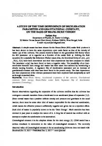
Figure 2: The deceleration parameter q(z) is reconstructed for the parametrization given by equation (23) using different values of N, as indicated in the each panel. The central thick line (black) represents the best-fit curve, while the dashed and dotted contours represent the 1σ and 2σ confidence level respectively. In each panel, the orange, red and magenta lines represent the trajectory of q for the Model 2, 3 and the ΛCDM model (with ΩΛ0 = 0.73) respectively. Also, the horizontal thin line indicates q(z) = 0.
11
0.5
0.0 N =2 N =3
q
N =4
-0.5 N =5 LCDM Model 2
-1.0
Model 3
-1.5 0
1
2
3
4
5
z
Figure 3: Evolution of q(z) is shown upto z > −1 for various models using the best-fit values of q0 and q1 arising from the joint analysis of SNIa+BAO/CMB dataset (see table 1 & 2). 0.0
-0.2 N =2
Ω tot
-0.4
N =3 N =4
-0.6 N =5
-0.8 -1.0 -1.2 0
1
2
3
4
5
z
Figure 4: The reconstructed total EoS parameter ωtot (z) for the best-fit model by considering different values of N, as indicated in the panel (see also Table 1). them in table 3. This results are found to be consistent with the results obtained by many authors from different considerations [14, 19]. For comparison, the corresponding curves for the Model 2, Model 3 and the ΛCDM model are also plotted in figure 2 which shows that the evolution of q(z) is not always compatible with Model 2 for different choices of N. It is also clear from figure 2 that the best fit values of q0 and zt are in good agreement with the standard ΛCDM model (within 2σ errors) and the Model 3 (within 1σ confidence level) if we increase the value of N. From figure 3, it is seen that as z approaches −1, the evolution of q(z) deviates from that of ΛCDM model. Such a behavior of q(z) may be an outcome of the choice “κ = ln N” made in equation (23). As mentioned earlier, the choice of κ = ln N was made such that q0 provides the present value of deceleration parameter. Some other choice of κ may as well be made so as to make ΛCDM model consistent in far future and thus needs more detailed analysis. The best fit evolution of the total EoS parameter ωtot as a function of z, given by equation (29), is shown in figure 4, which indicates that ωtot attains the required value of − 13 at z < 1 (or, at z < 1.4 for N = 2) and remains greater than −1 up to the current epoch (i.e., z = 0) for the combined (SNIa+BAO/CMB) dataset. This result is consistent with the recent observational results. On the other hand, figure 5 clearly shows the departure of j, given by
12
1.4
jHzL
1.2
1.0 N =2 N =3
0.8
N =4 N =5 LCDM
0.6
0.4 0
1
2
3
4
5
z
Figure 5: The evolution of j(z) with respect to redshift z is shown using the best-fit values of q0 and q1 for different values of N, as indicated in the frame. The horizontal thick line (magenta) indicates j = 1 (constant) for a ΛCDM model. equation (30), from the flat ΛCDM model ( j = 1) for the best-fit model. It is seen from figure 5 that for the best-fit model, the present value of j is greater than 1 for N = 3, 4 and 5, while for N = 2, j is less than 1 (see also Table 3). So, the present model (with j 6= 1 and q0 < 0) clearly indicates that a dynamical DE is more likely to be responsible for the current acceleration. For statistical comparison of Model 1 with the Models 2 & 3, two model selection criterion have been used, the Akaike information criterion (AIC) and the Bayesian Information Criterion (BIC). The AIC is defined as [43] AIC = −2lnLmax + 2g (44) and the BIC is defined as [44] BIC = −2lnLmax + glnk
(45)
where, Lmax is the maximum likelihood (equivalently, minimum of χ 2 ) obtained for the model, g is the number of free parameters in that model and k is the number of data points used for the data analysis. If the magnitude of the differences between the AIC (△AIC) of the two models (or △BIC) is less than 2, then the toy model under consideration (here, Model 1) is strongly favored by the reference model (here, Models 2 & 3). On the other hand, if the magnitude of △AIC or △BIC is greater than 10, then the models strongly disfavor each other. As mentioned earlier, the statistical analysis is done by fixing the parameter N to some constant. Because of this, all the three models (Models 1, 2 & 3) have same number of degrees of freedom, and thus △AIC or △BIC will be same. Now for Model 1 in comparison with the Model 2 and 3, the △AIC (or △BIC) values are given by 2 2 △AIC = χmin (Model 1) − χmin (Model 2)
and 2 2 △AIC = χmin (Model 1) − χmin (Model 3)
Now, it is clear from table 1 and 2 that for the model 3, the △AIC (or △BIC) is less than 2 for each choices of N. Hence, the present reconstructed model is highly consistent with the model 3.
13
4 Conclusions In the present work, we have studied the dynamics of accelerating scenario within the framework of scalar field model. Here, we have considered one specific parameterization of the deceleration parameter q(z) and from this we have found out analytical solutions for various cosmological parameters. As we have seen before, the new parametrization of q(z) is similar to the well-known parametrization of q(z) for appropriate choices of q0 , q1 and N. We have also compared our thez oretical model with three different popular models, such as q ∝ z (see equation (31)), q ∝ 1+z (see equation (33)) and ΛCDM (see equation (35)), to draw a direct comparison between them. In what follows, we have summarized the main results of our analysis. The observational data analysis by χ 2 -minimization technique have also been analyzed for this model using the SNIa+BAO/CMB dataset. From this analysis, we have obtained the bounds on the arbitrary parameters q0 and q1 within 1σ and 2σ confidence levels. It has been found that q(z) shows exactly the behavior which is desired, a deceleration for high z limit whereas an acceleration for the low z limit. This is essential to explain both these observed growth of structure at the early epoch and the late-time cosmic acceleration measurements. It should be noted that for the present model, the values of the transition redshift zt with 1σ errors are consistent with the values obtained by many authors from different scenarios [14, 19]. For this model, the jerk parameter j is found to be evolving, which indicates a tendency of deviation of the universe from the standard ΛCDM model. These results make the present work worthy of attention. The present model also provides an analytical solution for the EoS parameter ωφ (z). Interestingly, it has been found that the EoS parameter reduces to the well-known CPL parametrization of ωφ (z) for low z [32, 33]. To obtain more physical insight regarding the evolution of ωφ (z), we have plotted the reconstructed total EoS parameter in figure 4 and the resulting scenarios agree very well with the observational results at the present epoch. As discussed earlier, this particular choice of q(z) is quite arbitrary and we have made this assumption to close the system of equations. Since the nature of the universe is still a mystery, therefore the idea to parameterize q(z) is a simple approach to study the transition of the universe from decelerated to accelerated expansion phase and also opens up possibilities for future studies regarding the nature of dark energy. Definitely, the addition of more observational datasets in the present work may help us to obtain more precise constraints on the expansion history of the universe and the present work is one preliminary step towards that direction.
5 Acknowledgements The authors are thankful to the anonymous referee whose useful suggestions have improved the quality of the paper. A.A.M. acknowledges UGC, Govt. of India, for financial support through a Maulana Azad National Fellowship. SD wishes to thank IUCAA, Pune for associateship program.
References [1] A. G. Riess et al., Astron. J., 116, 1009 (1998). [2] S. Perlmutter et al., Astrophys. J., 517, 565 (1999).
14 [3] S. Weinberg, Rev. Mod. Phys., 61, 1 (1989). [4] P. J. Steinhardt et al., Phys. Rev. Lett., 59, 123504 (1999). [5] E. J. Copeland, M. Sami and S. Tsujikawa, Int. J. Mod. Phys. D, 15, 1753 (2006). [6] L. Amendola and S. Tsujikawa, Dark energy-Theory and observations, Cambridge University Press (2010). [7] M. S. Turner and A. G. Riess, Astrophys. J., 569, 18 (2002). [8] A. G. Riess et al., Astrophys. J., 607, 665 (2004). [9] Y. G. Gong and A. Wang, Phys. Rev. D, 73, 083506 (2006). [10] Y. Gong and A. Wang, Phys. Rev. D, 75, 043520 (2007). [11] J. V. Cunha and J. A. S. Lima, MNRAS, 390, 210 (2008). [12] J. V. Cunha, Phys. Rev. D, 79, 047301 (2009). [13] B. Santos et al., arXiv:1009.2733 [astro-ph.CO]. [14] R. Nair et al. JCAP, 01, 018 (2012) [arXiv:1109.4574 [astro-ph.CO]]. [15] O. Akarsu et al., EPJ Plus, 129, 22 (2014). [16] L. Xu and H. Liu, Mod. Phys. Lett. A, 23, 1939 (2008). [17] L. Xu and J. Lu, Mod. Phys. Lett. A, 24, 369 (2009). [18] S. del Campo et al., Phys. Rev. D, 86, 083509 (2012). [19] A. A. Mamon and S. Das, Int. J. Mod. Phys. D, 25, 1650032 (2016). [20] A. Shafieloo, Mon. Not. Roy. Astron. Soc., 380, 1573 (2007). [21] T. Holsclaw et al., Phys. Rev. D, 82, 103502 (2010). [22] T. Holsclaw et al., Phys. Rev. D, 84, 083501 (2011). [23] R. G. Crittenden et al., JCAP, 02, 048 (2012). [24] R. Nair, S. Jhingan and D. Jain, JCAP, 01, 005 (2014). [25] V. Sahni and A. A. Starobinsky, Int. J. Mod. Phys. D, 15, 2105 (2006). [26] M. Visser, Class. Quant. Grav., 21, 2603 (2004). [27] O. Luongo, Mod. Phys. Lett. A, 19, 1350080 (2005). [28] D. Rapetti, S. W. Allen, M. A. Amin and R. D. Blandford, Mon. Not. Roy. Astron. Soc., 375, 1510 (2007).
15 [29] R. D. Blandford et al., ASP Conf. Ser., 339, 27 (2004) [astro-ph/0408279]. [30] V. Sahni, T. D. Saini, A. A. Starobinsky, U. Alam, JETP Lett., 77, 201 (2003). [31] U. Alam, V. Sahni, T. D. Saini, A. A. Starobinsky, MNRAS, 344, 1057 (2003). [32] M. Chevallier and D. Polarski, Int. J. Mod. Phys. D, 10, 213 (2001). [33] E. V. Linder, Phys. Rev. Lett., 90, 091301 (2003). [34] Jing-Zhe Ma and Xin Zhang, Phys. Lett. B 699, 233 (2011) [ arXiv:1102.2671 [astro-ph.CO]]. [35] M. Betoule et al., Astron. Astrophys., 568, A22 (2014). [36] O. Farooq, D. Mania and B. Ratra, Astrophys. J., 764, 138 (2013). [37] C. Blake et al., Mon. Not. R. Astron. Soc., 418, 1707 (2011). [38] N. Padmanabhan et al., Mon. Not. Roy. Astron. Soc., 427, 2132 (2012). [39] L. Anderson et al., Mon. Not. Roy. Astron. Soc., 427, 3435 (2013). [40] F. Beutler et al., Mon. Not. R. Astron. Soc., 416, 3017 (2011). [41] P. A. R. Ade et al. [Planck Collaborations], A&A, 594, A13 (2016). [42] M. V. dos Santos et al., JCAP, 02, 066 (2016). [43] H. Akaike, IEEE Trans. Autom. Control., 19, 716 (1974). [44] G. Schwarz, Ann. Stat., 6, 461 (1978).