Abstract. We present an algorithm for causal structure discovery suited in the presence of continuous variables. We test a version based on partial correlation ...
A Partial Correlation-Based Algorithm for Causal Structure Discovery with Continuous Variables Jean-Philippe Pellet1,2 and Andr´e Elisseeff1 1
IBM Research Business Optimization Group S¨ aumerstr. 4, 8803 R¨ uschlikon, Switzerland {jep,ael}@zurich.ibm.com 2
Swiss Federal Institute of Technology Zurich Machine Learning Group Institute of Computational Science Universit¨ atstr. 6, 8092 Zurich, Switzerland
Abstract. We present an algorithm for causal structure discovery suited in the presence of continuous variables. We test a version based on partial correlation that is able to recover the structure of a recursive linear equations model and compare it to the well-known PC algorithm on large networks. PC is generally outperformed in run time and number of structural errors.
1
Introduction
Detecting causation from observational data alone has long been a controversial issue. It is not before the pioneering work of Pearl and Verma [1] and Spirtes et al. [2] that causal discovery was formalized theoretically and linked with a graphical representation: directed acyclic graphs (DAGs). PC,3 the reference causal discovery algorithm, is based on conditional independence (CI) tests. While such a test can be implemented efficiently with discrete variables, it is not generalizable to the continuous case straightforwardly. With the assumption that variables are jointly distributed according to a multivariate Gaussian, we know that a test for zero partial correlation4 is equivalent to a CI test [3]. In this paper, we present an algorithm based on partial correlation that is faster and makes fewer errors than PC on datasets with more than a few hundred samples. In section 2, we review principles of causal discovery, pose the problem, and mention related work. We then present the algorithm in section 3 and analyze its complexity. Experimental results are shown and discussed in section 4. We conclude in section 5 and include proofs and definitions in appendix A. 3 4
“PC” stands for “Peter” and “Clark” after the inventors of the method [2]. Definition in appendix A.
2
Background & Problem Statement
The search for the true causal structure underlying some data set is of paramount importance when the effect actions rather than predictions are to be returned. By focusing on predictions only, a system cannot address problems where some parts of the data distribution process is changed. Causality analysis is a mean to address these nonstationary problems by computing the mechanism generating the data and by assessing the effect of some changes in that mechanism. The first step to a causal analysis is the definition of the causal structure represented as a DAG. In general, this problem is impossible to solve with observational data only. Causal structures can be retrieved only up to some equivalence class: besides (undirected) adjacencies, only colliders, i.e., triples of variables where one is a common effet of two causes, can be specified exactly. There are mainly two classes of causal discovery algorithms: score-based and constrained-based. In this paper, we are concerned with the second type only. PC is a typical constraint-based algorithm. We present its high-level description, also known as the IC algorithm [1]: 1. For each variable pair (X, Y ) in the set of variables V, look for a set SXY such that X and Y are conditionally independent given SXY : (X ⊥ ⊥ Y | SXY );5 add an edge between X and Y if no such set can be found; 2. For each pair (X, Y ) with a common neighbor Z, turn the triple into a V-structure X → Z ← Y if Z ∈ SXY ; 3. Propagate the arrow orientation to preserve acyclicity without introducing new V-structures. Because of the subset search in Step 1, PC and IC have an exponential time complexity in the worst case. Current causal discovery algorithms assume that the underlying causal structure is a Bayesian network (with discrete variables), i.e., that the dataset is DAG-isomorphic [4]. Extensions have been developed for the case of continuous variables when the underlying causal structure is a linear structural equation model (SEM). In SEMs, we describe each variable xi = fi (pai , ui ) as a function of its parents and a random disturbance term. When the corresponding graph is acyclic, the SEM is said to be recursive. In this paper, we focus on SEMs and on continuous variables, frequent in econometrics, social sciences, and health care, for instance. Focusing on SEMs rather than Bayesian networks avoids the computational difficulties of handling continuous conditional probability distributions. But one of the main challenges to solve is to find a convincing statistical test of CI for continuous variables. To simplify our task, we solve the simpler case of a linear recursive SEM, where each functional equation is of the form xi = hwi , pai i + ui . Imposing a Gaussian distribution on the disturbance terms ui yields a multivariate Gaussian distribution ⊥ Y | Z) over V, and a partial correlation ρXY ·Z will be zero if and only if (X ⊥ 5
We have (X ⊥ ⊥ Y | Z ) ⇐⇒ P (X = x | Z = z) = P (X = x | Y = y, Z = z).
holds. Thus, testing for zero partial correlation is a valid conditional independence test for continuous variables in a linear recursive SEM with uncorrelated Gaussian disturbance terms. Related Work Partial correlation has been used extensively in econometrics and social sciences in path analysis with relatively small models (e.g., [5]). In causal discovery, it has only been used (as transformed by Fisher’s z, see [6, 7]) as a continuous replacement for CI tests designed for discrete variables and assuming a small conditioning set size. Causal graph construction, especially if considered as determination of the Markov blanket of each variable, can be assimilated to a feature selection task for each node. Other causal algorithms performing a search to retrieve the Markov blanket of single variables include MMMB [8] and HITON MB [9]. These papers also discuss the link to feature selection. But to the best of our knowledge, none of them has been extended and applied to fully-continuous datasets. Other approaches to learning the structure of causal or Bayesian networks with continuous variables without first discretizing them include using a CI test from Margaritis [10]. This test, however, is very computationally expensive, which limits its use even for medium-sized problems. Work has also been done in score-based approaches for learning with continuous [11] and mixed [12] variables and integrating expert knowledge in the form of priors, but they do not provide a theoretical proof that the obtained graph is a perfect map of the dataset.
3
Total Conditioning for Causal Discovery
Whereas PC removes edges from a full graph as CI is found, our Total Conditioning (TC) method starts with an empty graph and adds edges between two nodes when conditioning on all the others does not break any causal dependency. 1. For each pair (X, Y ), add an edge X−Y if the partial correlation ρXY ·V\{X,Y } does not vanish. We obtain the moral graph of G0 , i.e., an undirected copy of G0 where all parents of the colliders are pairwise linked; 2. Remove spurious links between parents of colliders introduced in Step 1 and identify V-structures; 3. Propagate constraints to obtain maximally oriented graph (completed PDAG). Partial correlations in Step 1 can be computed efficiently by inverting the √ correlation matrix R. With R−1 = (rij ), we have: ρXi Xj ·V\{Xi ,Xj } = −rij / rii rjj . In terms of Gaussian Markov random fields (a special case of undirected graphical models), Step 1 constructs the correct graph by adding edges where the total partial correlation is significantly different from zero (see, e.g., [13]). In the case of the DAG-isomorphic problems we handle, Step 1 builds the correct structure up to moral graph equivalence: it will actually build the correct undirected links and marry all parents. This means that every original V-structure will be turned into a triangle pattern. Step 3 is common to several algorithms
constructing the network structure under CI constraints [1, 2]. Step 2 is a local search looking for orientation possibilities. To explain it, we need the following definition. Definition 1. In an undirected graph G = (V, E), let Tri(X − Y ) (with X, Y ∈ V and (X, Y ) ∈ E) be the set of vertices forming a triangle with X and Y . Suppose that G is the moral graph of the DAG representing the causal structure of some DAG-isomorphic dataset. A set of vertices Z ⊂ Tri(X − Y ) then has the Collider Set property for the pair (X, Y ) if it is the largest set that fulfills ∃SXY ⊂ V \ {X, Y } \ Z : (X ⊥ ⊥ Y | SXY ) and
∀Zi ∈ Z : (X ⊥ 6 ⊥ Y | SXY ∪ Zi ) .
(1) (2)
Step 2 looks at each edge that is part of some triangle and determines if it is spurious due to a V-structure effect. This is exactly the case when two variables X, Y in a triangle X, Y, Z can be made conditionally independent by a set that does not contain Z. A search is then performed for each of those edges to determine a set Z ⊂ Tri(X − Y ) that has the Collider Set property, using a small search space for SXY and Z as allowed by the result of Step 1. If this search is successful, the edge X − Y is removed and the detected V-structures properly oriented for each collider. Practically, the search for SXY can be restricted to a subset of the union of the Markov blankets for X and Y , and the search for Z is restricted by definition to Tri(X − Y ), which make both tasks tractable, unless the graph has a high connectedness.
Algorithm 1 The Total Conditioning algorithm Input: D : p × n dataset with p n-dimensional data points Output: G : maximally oriented partially directed acyclic graph 1: 2: 3: 4: 5: 6: 7: 8: 9: 10: 11: 12:
G ← empty graph with n nodes for each unordered pair X, Y do if ρXY ·V\{X,Y } does not vanish then add link Y − X to G end for for each edge X − Y part of a fully-connected triangle do if ∃Z ⊂ Tri(X − Y ) that satisfies the Collider Set property then remove link X − Y from G for each Zi ∈ Z do orient edges as X → Zi ← Y end if end for perform constraint propagation on G to obtain completed PDAG return G
Complexity Analysis Step 1 has a complexity of O(n3 ), which comes from the matrix inversion needed to compute the partial correlations. Step 2 has a complexity O(n2 2α ), where α = maxX,Y |Tri(X − Y )| − 1. Step 3 is O(n3 ). The
overall complexity is then O(n3 + n2 2α ), depending on the value of α as determined by the structure of the graph to be recovered. In the worst case of a fully-connected graph, it is, like PC, exponential in the number of variables. After removal of the spurious links and the usual constraint propagation [1, 2], the returned graph is the maximally-oriented PDAG of the Markov equivalence class of the generating DAG G0 . In the appendix, we prove the correctness of TC; i.e., we show that in the large-sample limit and with reliable statistical tests, TC converges to the actual perfect map of the dataset to be analyzed, up to its equivalence class. Significance Tests A particularly delicate point in this algorithm is the statistical test deciding whether a partial correlation is significantly different from zero. In a network of n nodes, Step 1 performs n(n − 1)/2 tests for determining the undirected skeleton. On average, we will then falsely reject the null hypothesis ρ = 0 about αn(n − 1)/2 times, and thus include as many wrong edges in the graph. We then set the significance level for the individual tests to be inversely proportional to n(n − 1)/2 to avoid this problem, without noticing an increase in the Type II error rate experimentally. The PC algorithm does not suffer from this issue because of the detailed way of repeatedly testing for edge existence with increasing conditioning set cardinality. In practice, we replaced the more traditional Fisher approximate z-transform of the sample correlation by t-tests on the beta weights of the corresponding linear regression equations, whose distributions are known to be Gaussian with zero mean under the null hypothesis ρ = 0 (see, e.g., [14], p. 243).
4
Experimental Results
The performance of the TC algorithm was evaluated against the PC algorithm [2] where CI tests were replaced by zero partial correlation tests. We were unable to compare it to newer algorithms like SCA [15] or MMHC [16] because generalizing them to handle continuous variables require techniques that are too computationally expensive. We used the following networks (from the Bayes net repository): – Alarm, 37 nodes, 46 arcs, 4 undirected in the PDAG of the equivalence class. It was originally designed to help interpret monitoring data to alert anesthesiologists to various situations in the operating room. – Hailfinder, 56 nodes, 66 arcs, 17 undirected in its PDAG. It is a normative system that forecasts severe summer hail in northeastern Colorado. – A subset of Diabetes, with 104 nodes, 149 arcs, 8 undirected in its PDAG, which was designed as a preliminary model for insulin dose adjustment. The graphs were used as a structure for a linear SEM. The parentless variables were sampled as Gaussians with zero mean and unit standard deviation; the other variables were defined as a linear combination of their parents with coefficient randomly distributed uniformly between 0.1 and 0.9, similarly to what
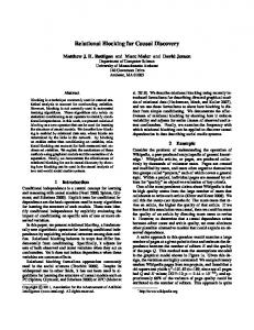
was done in [6]. The disturbance terms were also normally distributed. We used the implementation of PC proposed in the BNT Structure Learning Matlab package [17], where we set the statistical significance of the tests to α = 0.05. The implementation of TC was also done in Matlab; all experiments were run on a 2 GHz machine. Fig. 1 (a) shows the training errors for PC and TC against the number of samples for Alarm. For each sample size, 9 datasets were drawn from the model; the error bars picture the standard deviation over these 9 runs. Starting at about 150 samples, TC outperforms PC. It introduces at most one unnecessary arc and misses between 0 and 3. On average, TC was about 20 times faster than the implementation of PC we used, although the factor tended to decrease with larger sample sizes; see Fig. 1 (b). The results for Hailfinder are shown in Fig. 2. The results for PC are sparser than for TC, because of its long run times. In order to speed it up, we set the maximum node fan-in parameter to 6, so that PC would not attempt to conduct CI tests with conditioning sets larger than 6. For large datasets, we could run PC only once, so that we have little information on the variance of its results for this network, but even if we average the five last PC results for between 550 and 10000 samples, TC does better for each of its runs on this range. PC still beats TC on sample sizes smaller than 200. We also see on Fig. 2 (b) how the fan-in parameter imposed an upper bound on the run times of PC. Fig. 3 shows errors and run times for Diabetes (note that the sample size starts from 200, because in the case where we have fewer samples than the number of variables, TC would have to inverse a matrix that does not have full rank). Again, PC does better at first, and starting at 500 samples, it is outperformed in accuracy. The difference of the number of errors stabilizes around 5 or 6. Our run times are still significantly shorter. Finally, Fig. 4 shows the results of an experiment where we took the first n nodes of Diabetes for a fixed sample size of 1000 in order to show the response of the algorithms to an increasing number of variables in networks of similar structure. Results show that PC makes 1 to 2 mistakes fewer on the smaller networks but is outperformed for n > 50 on this particular instance. Although the run times of PC are still significantly higher, rescaling the plots shows that the increase of n increases the run times of both algorithms by a very similar factor for all tested graph sizes. Discussion TC consistently beats PC when the sample size gets larger, and does so in a small fraction of the time needed by PC. In particular, PC is slowed down by nodes with a high degree, whereas TC handles them without the exponential time complexity growth if they are not part of triangles, as in Hailfinder. In general, TC resolves all CI relations (up to married parents) in O(n3 ) in Step 1, whereas all PC can do in O(n3 ) is resolve CI relations with conditioning sets of cardinality 1. It is then reasonable to expect TC to scale better than PC on sparse networks where nodes have a small number of parents. PC could not be beaten on small sample sizes. It is yet an unsolved challenge for TC to handle problems where the number of variables exceeds the number of
(a)
(b)
25 TC PC
TC PC 5
4 Training time in s
Number of structural errors
20
15
10
5
3
2
1
0 2 10
0 2 10
3
10 Sample size
3
10 Sample size
Fig. 1. Alarm: (a) structural errors and (b) run times as a function of sample size
(a)
(b)
55 TC PC
50
TC
30
PC! 10!2
45 25
35
Training time in s
Structural errors
40
30 25 20
20
15
10
15 10
5
5 0 2 10
0 2 10
3
10 Sample size
3
10 Sample size
Fig. 2. Hailfinder: (a) structural errors and (b) run times as a function of sample size
(b)
(a) 70 TC PC 60
80 70 Training time in s
50 Structural errors
TC PC
90
40
30
60 50 40 30
20
20 10
0 250
10
3
4
10
10 Sample size
0
250
3
4
10
10 Sample size
Fig. 3. Diabetes: (a) structural errors and (b) run times as a function of sample size
(b)
(a) 300
15
TC PC
TC PC
200
10 Run time in s
Number of structural errors
250
150
100
5
50
0
10
20
30
40 50 60 70 Graph size in nodes
80
90
100
0
10
20
30
40 50 60 70 Graph size in nodes
80
90
100
Fig. 4. Diabetes: (a) structural errors and (b) run times as a function of n
samples, as in gene expression networks, thus leading to an attempt at inverting a matrix that does not have full rank. Regularizing the covariance matrix might help make TC more robust in this case. PC and TC are complementary in the sense that PC is preferably used with smaller sample sizes, and TC can take over more accurately with larger datasets.
5
Conclusion
Causal discovery with continuous variables is tractable with the multivariate Gaussian assumption and partial correlation: we showed an algorithm based on it to recover the exact structure in the large sample limit. The algorithm first checks for each pair of variables if their association can be accounted for by the intermediate of other variables, and if not, links them, thus determining the Markov blanket of each node. A second pass performs a local search to detect the V-structure and orient the graph correctly. The proposed algorithm outperforms or equals the reference PC algorithm in accuracy (except for very small sample sizes) in a fraction of its run time. In the future, we intend to investigate further the behavior of the algorithm and improve it in these conditions. We will also work on generalizing partial correlation and the underlying linear regression to the nonlinear case.
A
Appendix: Correctness Proof
For all proofs, we assume the given dataset D is DAG-isomorphic. Definition 2. Partial correlation between variables X and Y given a set of variables Z is the correlation of the residuals RX and RY resulting from the linear regression of X on Z and of Y on Z, respectively.
Definition 3. In an DAG G, two nodes X, Y are d -separated by Z ⊂ V \ {X, Y }, written (X ↔ | Y | Z ), if every path from X to Y is blocked by Z. A path is blocked if at least one diverging or serially connected node in in Z or if at least one converging node and all its descendants are not in Z. If X and Y are not d-separated by Z, they are d-connected: (X ↔ Y | Z ). This is generalized to sets X, Y: (X ↔ | Y | Z ) holds if pairwise separation holds for all i, j: (Xi ↔ | Yj | Z ). Lemma 1. In a DAG G, any (undirected) path π of length `(π) > 2 can be blocked by conditioning on any two consecutive nodes in π. Proof. It follows from Def. 3 that a path π is blocked when either at least one collider (or one of its descendants) is not in S, or when at least one non-collider is in S. It therefore suffices to show that conditioning on two consecutive nodes always includes a non-collider. This is the case because two consecutive colliders would require bidirected arrows, which is a structural impossibility with simple DAGs. t u Lemma 2. In a DAG G, two nodes X, Y are d-connected given all other nodes S = V \ {X, Y } if and only if any of the following conditions holds: (i) There is an arc from X to Y or from Y to X (i.e., X → Y or X ← Y ); (ii) X and Y have a common child Z (i.e., X → Z ← Y ). Proof. We prove this by first proving an implication and then its converse. (⇐=) If (i) holds, then X and Y cannot be d -separated by any set. If (ii) holds, then Z is included in the conditioning set and d -connects X and Y by Def. 3. (=⇒) X and Y are d -connected given a certain conditioning set when at least one path remains open. Using the conditioning set S, paths of length > 2 are blocked by Lemma 1 since S contains all nodes on those paths. Paths of length 2 contain a mediating variable Z between X and Z; by Def. 3, S blocks them unless Z is a common child of X and Y . Paths of length 1 cannot be blocked by any conditioning set. So the two possible cases where X and Y will be d -connected are (i) or (ii). t u Corollary 1. Two variables X, Y are dependent given all other variables S = V \ {X, Y } if and only if any of the following conditions holds: (i) X causes Y or Y causes X; (ii) X and Y have a common effect Z. Proof. It follows directly from Lemma 2 due to the DAG-isomorphic structure, which ensures that there exists a DAG where CI and d -separation map oneto-one. Lemma 2 can then be reread in terms of CI and causation instead of d -separation and arcs. t u Lemma 3. The subset Z that has the Collider Set property for the pair (X, Y ) is the set of all direct common effects of X and Y and exists if and only if X is neither a direct cause nor a direct effect of Y .
Proof. The fact that Z exists if and only if X is neither a direct cause nor a direct effect of Y is a direct consequence of (1), which states that X and Y can be made conditionally independent. This is in contradiction with direct causation. We now assuming that some SXY and Z have been found. (=⇒) By (1) and (2), we know that each Zi opens a dependence path between X and Y (which are independent given SXY ) by conditioning on SXY ∪ Zi . By Def. 3, conditioning on Zi opens a path if Zi is either a colliding node or one of its descendants. As, by definition, Z ⊂ Tri(X − Y ), we are in the first case. We conclude that Zi is a direct effect of both X and Y . (⇐=) Note that (1) and (2) together are implied in presence of a V-structure X → Zi ← Y . Thus, a direct effect is compatible with the conditions. The fact that Z captures all direct effects follows from the maximization of its cardinality. t u Theorem 1. If the variables are jointly distributed according to a multivariate Gaussian, TC returns the PDAG of the Markov equivalence class of the DAG representing the causal structure of the data-generating process. Proof. An edge is added in Step 1 between X and Y if we find that ρXY ·V\{X,Y } 6= 0. We conclude (X ⊥ 6 ⊥ Y | V \ {X, Y } ), owing to the multivariate Gaussian distribution. Corollary 1 says that this implies that X causes Y or Y causes X, or that they share a common child. Therefore, each V-structure is turned into a triangle by Step 1. Step 2 then examines each link X − Y part of a triangle, and by Lemma 3, we know that if the search for a set Z that has the Collider Set property succeeds, there must be no link between X and Y . We know by the same lemma that this set includes all colliders for the pair (X, Y ), so that all V-structures are correctly identified. Step 3 is the same as in the IC or PC algorithms; see Pearl and Verma [1, 2]. t u
References 1. Pearl, J., Verma, T.: A theory of inferred causation. In: Proc. of the Second Int. Conf. on Principles of Knowledge Representation and Reasoning, Morgan Kaufmann (1991) 2. Spirtes, P., Glymour, C., Scheines, R.: Causation, Prediction, and Search. Volume 81. Springer Verlag, Berlin (1993) 3. Baba, K., Shibata, R., Sibuya, M.: Partial correlation and conditional correlation as measures of conditional independence. Australian & New Zealand Journal of Statistics 46(4) (2004) 4. Wong, S.K.M., Wu, D., Lin, T.: A structural characterization of dag-isomorphic dependency models. In: Proc. of the 15th Conf. of the Canadian Society for Computational Studies of Intelligence, Morgan Kaufmann (2002) 195–209 5. Alwin, D.F., Hauser, R.M.: The decomposition of effects in path analysis. American Sociological Review, 40(1) (1975) 6. Scheines, R., Spirtes, P., Glymour, C., Meek, C., Richardson, T.: The tetrad project: Constraint based aids to causal model specification. Technical report, Carnegie Mellon University, Dpt. of Philosophy (1995)
7. Sch¨ afer, J., Strimmer, K.: Learning large-scale graphical gaussian models from genomic data. In: AIP Conference Proceedings 776. (2005) 263–276 8. Tsamardinos, I., Aliferis, C., Statnikov, A.: Time and sample efficient discovery of markov blankets and direct causal relations. In: Proc. of the 9th ACM SIGKDD Int. Conf. on Knowledge Discovery and Data Mining. (2003) 9. Aliferis, C.F., Tsamardinos, I., Statnikov, A.: Hiton, a novel markov blanket algorithm for optimal variable selection. In: Proceedings of the 2003 American Medical Informatics Association (AMIA) Annual Symposium. (2003) 21–25 10. Margaritis, D.: Distribution-free learning of bayesian network structure in continuous domains. In: Proc. of the 20th National Conf. on AI. (2005) 11. Geiger, D., Heckerman, D.: Learning gaussian networks. Technical Report MSRTR-94-10, Microsoft Research (1994) 12. Bøttcher, S.: Learning bayesian networks with mixed variables. In: Proceedings of the Eighth International Workshop in Artificial Intelligence and Statistics. (2001) 13. Talih, M.: Markov Random Fields on Time-Varying Graphs, with an Application to Portfolio Selection. PhD thesis, Hunter College (2003) ˜ 1 tkepohl, H., Lee, T.C.: Introduction 14. Judge, G.G., Hill, R.C., Griffiths, W.E., LA 4 to the Theory and Practice of Econometrics, 2nd Edition. Wiley (1988) 15. Friedman, N., Linial, M., Nachman, I., Pe’er, D.: Using bayesian networks to analyze expression data. In: RECOMB. (2000) 127–135 16. Tsamardinos, I., Brown, L.E., Aliferis, C.F.: The max-min hill-climbing bayesian network structure learning algorithm. Machine Learning (2006) 17. Leray, P., Fran¸cois, O.: Bnt structure learning package (2004)