Page 1 ... estimates is the expectation-maximization (EM) algorithm. ... EM algorithm are specific to a given causal independence model, and hence not.
EM Algorithm for Symmetric Causal Independence Models Rasa Jurgelenaite and Tom Heskes Institute for Computing and Information Sciences, Radboud University Nijmegen, Toernooiveld 1, 6525 ED Nijmegen, The Netherlands {rasa, tomh}@cs.ru.nl
Abstract. Causal independence modelling is a well-known method both for reducing the size of probability tables and for explaining the underlying mechanisms in Bayesian networks. In this paper, we present the EM algorithm to learn the parameters in causal independence models based on the symmetric Boolean function. The developed algorithm enables us to assess the practical usefulness of the symmetric causal independence models, which has not been done previously. We evaluate the classification performance of the symmetric causal independence models learned with the presented EM algorithm. The results show the competitive performance of these models in comparison to noisy OR and noisy AND models as well as other state-of-the-art classifiers.
1
Introduction
Bayesian networks [1] are well-established as a sound formalism for representing and reasoning with probabilistic knowledge. However, because the number of conditional probabilities for the node grows exponentially with the number of its parents, it is usually unreliable if not infeasible to specify the conditional probabilities for the node that has a large number number of parents. The task of assessing conditional probability distributions becomes even more complex if the model has to integrate expert knowledge. While learning algorithms can be forced to take into account an expert’s view, for the best possible results the experts must be willing to reconsider their ideas in light of the model’s ‘discovered’ structure. This requires a clear understanding of the model by the domain expert. Causal independence models [2], [3], [4] can both limit the number of conditional probabilities to be assessed and provide the ability for models to be understood by domain experts in the field. The main idea of causal independence models is that causes influence a given common effect through intermediate variables and interaction function. Causal independence assumptions are often used in practical Bayesian network models [5], [6]. However, most researchers restrict themselves to using only the logical OR and logical AND operators to define the interaction among causes. The resulting probabilistic submodels are called noisy OR and noisy AND; their underlying assumption is that the presence of either at least one cause or all
causes at the same time give rise to the effect. Several authors proposed to expand the space of interaction functions by other symmetric Boolean functions: the idea was already mentioned but not developed further in [7], analysis of the qualitative patterns was presented in [8], and assessment of conditional probabilities was studied in [9]. Even though for some real-world problems the intermediate variables are observable (see [10]), in many problems these variables are latent. Therefore, conditional probability distributions depend on unknown parameters which must be estimated from data, using maximum likelihood (ML) or maximum a posteriori (MAP). One of the most widespread techniques for finding ML or MAP estimates is the expectation-maximization (EM) algorithm. Meek and Heckerman [7] provided a general scheme how to use the EM algorithm to compute the maximum likelihood estimates of the parameters in causal independence models assumed that each local distribution function is collection of multinomial distributions. Vomlel [11] described the application of the EM algorithm to learn the parameters in the noisy OR model. However, the proposed schemes of the EM algorithm are specific to a given causal independence model, and hence not directly applicable to the general case of parameter learning in causal independence models. Learning the parameters in causal independence models with a symmetric Boolean function as an interaction function (further referred to as the symmetric causal independence models) is the main topic of this paper. We develop an EM algorithm to learn the parameters in symmetric causal independence models. The presented algorithm enables us to assess the practical usefulness of this expanded class of causal independence models, which has not been done by other authors. The evaluation is done by using the symmetric causal independence models learned with the developed EM algorithm as classifiers. Experimental results show the competitive classification performance of these models in comparison with the noisy OR classifier as well as other widely-used classifiers. The remainder of this paper is organised as follows. In the following section, we review Bayesian networks and discuss the semantics of symmetric causal independence models. In Section 3, we first describe the general scheme of the EM algorithm and then develop the EM algorithm for finding the parameters in symmetric causal independence models. Section 4 presents the experimental results, and conclusions are drawn in Section 5.
2 2.1
Symmetric Boolean Functions for Modelling Causal Independence Bayesian Networks
A Bayesian network B = (G, Pr) represents a factorised joint probability distribution on a set of random variables V. It consists of two parts: (1) a qualitative part, represented as an acyclic directed graph (ADG) G = (V(G), A(G)), where there is a 1–1 correspondence between the vertices V(G) and the random variables in V, and arcs A(G) represent the conditional (in)dependencies between
the variables; (2) a quantitative part Pr consisting of local probability distributions Pr(V | π(V )), for each variable V ∈ V given the parents π(V ) of the corresponding vertex (interpreted as variables). The joint probability distribution Pr is factorised according to the structure of the graph, as follows: Y Pr(V) = Pr(V | π(V )) . V ∈V
Each variable V ∈ V has a finite set of mutually exclusive states. In this paper, we assume all variables to be binary; as an abbreviation, we will often use v + to denote V = > (true) and v − to denote V = ⊥ (false). We interpret > as 1 and ⊥ as 0 in an arithmetic context. An expression such as X g(H1 , . . . , Hn ) ψ(H1 ,...,Hn )=>
stands for summing g(H1 , . . . , Hn ) over all possible values of the variables Hk for which the constraint ψ(H1 , . . . , Hn ) = > holds. 2.2
Semantics of Symmetric Causal Independence Models
C1
C2
...
Cn
H1
H2
...
Hn
E
f
Fig. 1. Causal independence model.
Causal independence (also known as independence of causal influence) is a popular way to specify interactions among cause variables. The global structure of a causal independence model is shown in Figure 1; it expresses the idea that causes C1 , . . . , Cn influence a given common effect E through hidden variables H1 , . . . , Hn and a deterministic function f , called the interaction function. The impact of each cause Ci on the common effect E is independent of each other cause Cj , j 6= i. The hidden variable Hi is considered to be a contribution of the cause variable Ci to the common effect E. The function f represents in which way the hidden effects Hi , and indirectly also the causes Ci , interact to yield the final effect E. Hence, the function f is defined in such a way that when a relationship, as modelled by the function f , between Hi , i = 1, . . . , n, and E = > is satisfied, then it holds that f (H1 , . . . , Hn ) = >. It is assumed that Pr(e+ | H1 , . . . , Hn ) = 1 if f (H1 , . . . , Hn ) = >, and Pr(e+ | H1 , . . . , Hn ) = 0 if f (H1 , . . . , Hn ) = ⊥.
A causal independence model is defined in terms of the causal parameters Pr(Hi | Ci ), for i = 1, . . . , n and the function f (H1 , . . . , Hn ). Most papers on causal independence models assume that absent causes do not contribute to the effect [1]. In terms of probability theory this implies that it holds that Pr(h + i | − − ) = 1. In this paper we make | c ) = 0; as a consequence, it holds that Pr(h c− i i i the same assumption. In situations in which the model does not capture all possible causes, it is useful to introduce a leaky cause which summarizes the unidentified causes contributing to the effect and is assumed to be always present [12]. We model this leak term by adding an additional input Cn+1 = 1 to the data; in an arithmetic context the leaky cause is treated in the same way as identified causes. The conditional probability of the occurrence of the effect E given the causes C1 , . . . , Cn , i.e., Pr(e+ | C1 , . . . , Cn ), can be obtained from the causal parameters Pr(Hl | Cl ) as follows [4]: X
Pr(e+ | C1 , . . . , Cn ) =
n Y
Pr(Hi | Ci ) .
(1)
f (H1 ,...,Hn )=> i=1
In this paper we assume that the function f in Equation (1) is a Boolean function. n However, there are 22 different n-ary Boolean functions [13], [14]; thus, the potential number of causal interaction models is huge. However, if we assume that the order of the cause variables does not matter, the Boolean functions become symmetric [14] and the number reduces to 2n+1 . An important symmetric Boolean function is the exact P Boolean function ² l , n which has function value true, i.e. ²l (H1 , . . . , Hn ) = >, if i=1 ν(Hi ) = l with ν(Hi ) equal to 1, if Hi is equal to true and 0 otherwise. A symmetric Boolean function can be decomposed in terms of the exact functions ²l as [14]: f (H1 , . . . , Hn ) =
n _
²i (H1 , . . . , Hn ) ∧ γi
(2)
i=0
where γi are Boolean constants depending only on the function f . For example, for the Boolean function defined in terms of the OR operator we have γ0 = ⊥ and γ1 = . . . = γn = >. Another useful symmetric Boolean function is the threshold function τk , which simply checks whetherPthere are at least k trues among the arguments, n i.e. τk (H1 , . . . , Hn ) = >, if j=1 ν(Hj ) ≥ k with ν(Hj ) equal to 1, if Hj is equal to true and 0 otherwise. To express it in the Boolean constants we have: γ0 = · · · = γk−1 = ⊥ and γk = · · · = γn = >. Causal independence model based on the Boolean threshold function further will be referred to as the noisy threshold models. 2.3
The Poisson Binomial Distribution
Using the property of Equation (2) of the symmetric Boolean functions, the conditional probability of the occurrence of the effect E given the causes C1 , . . . , Cn
can be decomposed in terms of probabilities that exactly l hidden variables H1 , . . . , Hn are true, as follows: Pr(e+ | C1 , . . . , Cn ) =
X
0≤l≤n γl
X
n Y
Pr(Hi | Ci ) .
(3)
²l (H1 ,...,Hn ) i=1
Let l denote the number of successes in n independent trials, where pi is a probability of success in the ith trial, i = 1, . . . , n; let p = (p1 , . . . , pn ), then B(l; p) denotes the Poisson binomial distribution [15]: ( n ) l Y Y X pj z B(l; p) = (1 − pi ) . (4) 1 − p jz z=1 i=1 1≤j1