A Partition Detection System for Mobile Ad- Hoc Networks - CiteSeerX

A Partition Detection System for Mobile AdHoc Networks Hartmut Ritter, Rolf Winter, Jochen Schiller Institute of Computer Science Freie Universität Berlin, Germany {hritter, winter, schiller}@inf.fu-berlin.de Abstract— A vast amount of applications and mechanisms recently developed for mobile ad-hoc networks could greatly benefit from the utilization of network status information. That includes, but is not limited to the detection of network partitioning. Network partitioning is a form of network failure. A single connected network topology breaks apart into two or more network topologies separated from each other. Nodes within each partition are still able to communicate with each other but nodes in other partitions are unreachable. This paper proposes two different partition detection mechanisms, one using a centralized approach, the other one utilizing the advantages of a distributed mechanism. The simulations show that both approaches detect partitioning reliably, with both having unique advantages. Index Terms— partition detection, ad-hoc networks, network monitoring

I. INTRODUCTION

O

NE of the unique challenges in mobile ad-hoc networking environments is the phenomenon of network partitioning, which is the breakdown of a connected network topology into two or more separate, unconnected topologies. In fixed infrastructure based networks, the occurrence of network partition is highly unlikely and only possible if big parts of the infrastructure fail simultaneously. In mobile ad-hoc networks, the problem of partitioning can also occur due to the mobility of the participating nodes making it a more common phenomenon. Various applications and network services for mobile ad-hoc networks could benefit from a reliable partition detection mechanism. As an application, distributed mobile games are especially prone to network partition since they are expected to be played on the go. They are played, for example, while waiting for a bus or subway. Here often significant amounts of players move in a group and therefore partition the network. In such a situation it would be beneficial to detect the partitioning and not interpret it as node failure. This way two or more separate games can be established without having to restart a game. This special application area is considered to grow significantly during the next couple of years as a survey [1] conducted shows. In general applications which have to

perform expensive tasks in terms of network load on node failure would benefit from partition detection. If that node failure is due to a network partition, the application could choose to wait a certain amount of time expecting it to be a temporary phenomenon. This way the application could resume the normal operation after the network partition problem is solved without loading the network unnecessarily. Also, applications based on swarm intelligence can act and try to re-establish a fully connected network or they can intelligently adapt to the situation when using a partition detection system. A type of network service which would benefit is auto-configuration. When network partition takes place, a possibly big part of the network address space becomes available again in separate partitions and can therefore be reused. A network based on a topology control mechanism could also benefit from such an approach. On detection of network partitioning, the nodes could extend their transmission range to reconnect the separate network topologies. In this paper we compare two approaches to detect network partitioning, a centralized and a distributed approach. Both approaches have unique advantages which are compared and analyzed. The remainder of this paper is organized as follows. Section II discusses related work. Section III presents the network partitioning systems developed. In section IV both systems are analyzed on the basis of experimental results with the network simulator ns2 [2]. Section V concludes this paper and gives a brief outlook on our future work. II. RELATED WORK Especially the academic interest in group communication pushed for a partition detection scheme. Babaoglu et al. [3] developed a partitionable group communication service which allows so called “partition-aware applications” to operate in separated network topologies and, after two or more partitions merge, reconfigure themselves. The partitioning problem is handled by a simple PING/ACK mechanism. A node sends a PING message to another node. If it does not receive an ACK in a certain amount of time, that node is added to a list of suspects. A dynamic timeout mechanism is used which leads

to a reasonably accurate suspect list. This scheme lacks the ability to distinguish between node failure and partitioning which for most applications is desirable. Also it does not carefully choose the nodes that monitor the network to increase the detection probability. In general most of the schemes described here do not offer this important feature. Killijian et al. [4] go a step further and try to anticipate a network partition. They only briefly describe their system, which consists of 3 entities: a failure anticipator, a movement planner and an environment evaluator. Obviously these components heavily rely on some form of sensing equipment and a huge amount of information exchange. Especially the sensing equipment cannot be assumed for all participating nodes. This approach appears to be quite heavy weight and the authors do not mention how they intend to detect that partitioning has taken place. They also do not show any facts and figures that demonstrate the accuracy of their anticipation scheme. In [5] simple heartbeat messages are used. Partitioning is suspected in the absence of an expected heartbeat. Clearly, this scheme does not allow to distinguish between node failure and network partitioning. Other research conducted in the field of group communication explicitly includes the network partition problem [6][7]. These approaches show that they are resilient against the problems arising after a network breaks apart and eventually merges back together, but none of the approaches deal with the detection of the event itself. III. NETWORK PARTITION DETECTION Mobile ad-hoc networks based on radio technology such as Bluetooth [10] or wireless LAN [11] are restricted in terms of bandwidth and their multi hop capability. That limits the amount of participating nodes and the size of the network topology. In such networks we have the notion of borders due to their geographic constraints and their wireless nature. To be able to exploit this characteristic is important for the network partition detection system. Border nodes are especially suitable to play a vital role in the detection process. The general idea is that border nodes exchange messages among each other. This way they monitor large parts of the network. If the network breaks up into separate partitions the nodes cannot reach each other any more and therefore detect the partition. In order to be able to distinguish between failure of border nodes and partition, extra functionality is added. The network wide partition detection is complemented by a local monitoring mechanism to prevent false partition detection due to node failure. A. Common Functionality Both approaches we developed distinguish two sets of nodes. One set consists of nodes not actively taking part in the network partition detection system. The other set of nodes actively probes the network as part of the system. The nodes

probing the system have to be chosen carefully as mentioned above to ensure that most of the network topology is monitored. Their key property is that they have a relatively small amount of neighbors compared to the nodes not actively supporting the partition detection system. The prominent reason for this is because nodes with a relatively low neighbor count are most likely at the border of the network topology. The number of neighbors a node has allows us to select the most appropriate nodes for the active part of our system. In other words, it allows us to identify border nodes. Both approaches work in a way that nodes periodically send out beacon messages serving as keep-alive messages. Every active node monitors a certain amount of other active nodes (or just one in the centralized approach). If a beacon message from one of these monitored nodes is not overheard for a certain amount of time, network partition is suspected. Therefore, active nodes should be placed far apart so that the beacon messages travel through large parts of the network, thereby increasing the monitored network area. In order to distinguish whether the absence of the beacon is due to node failure or due to network partition, a local validation mechanism is used, as already mentioned. The nodes sending beacon messages elect a so called “buddy”. This buddy is a one hop neighbor monitoring the node sending the beacon message. If the buddy node cannot hear its one hop neighbor any more, it starts a route request for it. If it finds the node over a multi-hop path, it asks that node to elect a new buddy. If it does not find the node, it suspects node failure and notifies the other active nodes about that incidence. Using this buddy mechanism the probability for a false partition alarm is significantly reduced. It can be even further reduced by electing multiple buddies since a false partition alarm is only set off if all buddy nodes together with the active node fail simultaneously. Since the active node (or border node) identification is so important, we evaluated two different approaches here as well, a static one and a dynamic one, which adapts well to topology changes. Since the criteria for becoming an active node is the neighbor count, all nodes in the network have to monitor their immediate network neighborhood periodically. Every node sends a broadcast message with a time-to-live (in hops) of one so that the message is only heard by direct neighbors, which in turn send an acknowledgement. This way, every node always has a relatively up-to-date view of its immediate network environment. The static approach uses a fixed threshold. Here a node becomes active if it has equal or less neighbors than the threshold. In the dynamic approach, a node constantly piggybacks its own neighbor count onto application data packets. The receiving node extracts that information and generates a threshold based on the last set of neighbor counts received. If its own neighbor count is below that value, it becomes active. Nodes can also leave the active state again. When their

neighbor count increases, they stop actively taking part in the system. Since in mobile networks the network topology could constantly change and, therefore, the neighbor count could fluctuate, the system uses a kind of neighborhood hysteresis. That means that a node enters the active state at a certain neighbor count but returns to the inactive state at a neighbor count higher than the threshold to enter the active state (see Figure 1).

node state

active

not active number of neighbors Fig. 1. Neighborhood hysteresis

If an active node has only a few neighbors, there is a high probability that its neighboring nodes also have a relatively low neighbor count. It would be inefficient to activate those nodes since that area of the network topology is already covered. Both approaches make sure that nodes adjacent to active nodes do not become active themselves through a neighbor inquiry mechanism when joining the network, or by overhearing activation messages. The inquiry mechanism also makes sure that newly switched on nodes learn about beacon sources. Note, that the prerequisites for our system to work are that an efficient routing algorithm exists, which supports broadcast and unicast. Additionally, it should provide the ability to set a time to live field. B. Centralized Network Partition Detection The first system we developed takes a centralized approach. Only one of the active nodes sends out beacon messages periodically, with the other active nodes only being the endpoints for those messages. On start-up of the system, the first node that detects that it should become active sends out a broadcast message telling each node that it is the beacon source (or server). Conflict situations can be handled by an algorithm similar to the lowest ID algorithm [13] or by another clusterhead election procedure. Every subsequent node that becomes active sends a notification to that node causing it to periodically send out a beacon (unicast message) to the just activated border node. As long as all the border nodes receive the beacon periodically, the network between the border nodes and the beacon source is monitored and connected. This, again, is why the placement of the active

nodes is so important. If one of the border nodes does not hear the beacon any more, it would always interpret it as a result of network partition. That is why we introduce the local validation mechanism, which was already briefly mentioned. It works as follows. In the centralized approach only the beacon source elects a buddy on start-up. The buddy periodically sends out a PING message to the beacon source which responds to that message with an acknowledgement. It is important that the interval of this PING message is much smaller than the interval of the beacon message. This way node failure is detected much faster than partitioning and the monitoring border nodes can be notified before they suspect partition due to the absence of the beacon. When a new node within the network becomes active and registers at the server, the server sends out an updated list of all border nodes to the buddy. This way the buddy always has an up-to-date view of the partition detection system and knows which nodes it has to notify if the server fails and could also quickly replace the server on failure. Another approach would be to simply broadcast the failure message, instead of using unicast messages. We did not implement this approach, since we wanted to keep broadcasts to a minimum (see section V). Failing nodes are not the only source of disruption for the partition detection system. In a wireless network, messages are much more likely to fail than in a wired network. Therefore, partition detection mechanisms must be robust against an increased message failure rate. The border nodes do not expect every beacon message to arrive at their destination. Every border node allows a certain number of messages to be lost before they suspect network partition. If the allowed beacon message loss is for example 3 and the beacon interval is 10 seconds, the system would suspect partitioning after 30 seconds have passed without having received a beacon message and also not having received a failure notification from the server buddy. A similar mechanism is used for the keep-alive-messages exchanged between a buddy and the server. However, since they are one hop neighbors, message loss is considered to be far less significant. The border nodes that monitor the server have to send a keep-alive message back to the server infrequently to tell the server that they are still participating since they have no fail notification mechanism like the server does. That ensures that the server does not load the network unnecessarily after a border node failed. If a node changes its state to be inactive it notifies the server for the same reason. The centralized approach has one general disadvantage. The partition which contains the server does not detect the partition as such. This is because in the centralized approach active nodes do not exchange beacon messages amongst each other. Detecting partitioning in the server partition might not be necessary though. If the applications in all but one partition have to suspend their operation, the centralized approach is sufficient. This situation is described in the primary partition

model [8][9]. There is also one general case in which partitioning is not detected, neither in the centralized nor in the distributed approach. The algorithms will not detect a partitioning when a part of the network is separated that does not contain an active node. If the border node detection works properly, this can only occur if a very small amount of nodes are separated in a rather unlucky constellation. The question is whether someone would consider this a network partition. C. Distributed Network Partition Detection The distributed approach is in its operating mode similar to the centralized approach. One key difference is that every active node sends out beacon messages. On becoming an active node, the node sends out a broadcast message telling every other node that it just became active. Every node in the network, even the inactive ones, store a certain number of border node addresses together with the distances to those nodes in hops. If there are more addresses to store, the node either replaces “old” entries or it replaces addresses of nodes that are closer than the new node. When a node now becomes active, it uses these nodes as partner nodes. It sends a request to send beacon messages at a certain interval to them. With the active nodes already stored while having been inactive, a node becoming active already knows of other active nodes in the network and can directly participate in the system. The replacement strategy mentioned above ensures that large parts of the network are covered by the system since only the nodes furthest away are kept. Since every active node sends out beacon messages, they all need a buddy node. The buddy acts a similar way as in the centralized approach. A difference is that the active node always informs the buddy node when either a new partner node is chosen, or if a beacon requestor fails or is added. This way all other nodes (a small number of active nodes) that in some form interact with the active node get notified if it fails. The partner nodes then stop sending beacons and the beacon requestors have to choose a new partner for themselves. If active nodes get notified that one of their partner nodes failed, it can either choose to wait until a new node becomes active, or if too many partners fail, it could start a lookup request for active nodes to fill the partner table. The latter is especially useful after a partition was detected. There is one critical moment in the system on startup. When the detection system is initiated, the nodes start checking whether they should become active. That would lead to a broadcast storm shortly after startup. This is why nodes start a timer when they receive an activation broadcast. If that broadcast timer is not expired when they want to send their own activation broadcast, the nodes delay it until after the timer expires. This mechanism makes sure that the network is not loaded unnecessarily, keeps collisions to a minimum at startup and saves bandwidth for other packets such as application data packets. The distributed approach has one possible weak point. If a

buddy (or buddies if multiple exist) and its corresponding active node are separated by partitioning, the partition remains undetected in the case that the active node is the only active node in its partition. IV. EXPERIMENTAL RESULTS To validate the two approaches and to analyze their behavior and performance we implemented them using the ns2 network simulator. We evaluated four basic scenarios: • • • •

Networks without partition and failing nodes Networks with partitioning but without failing nodes Networks with failing nodes but without partitioning Networks with both failing nodes and partitioning

Additionally we changed parameters for the border node detection. Every scenario was simulated 50 times with a given parameter combination. The networks we simulated consisted of 50 nodes, which we believe is a reasonable number for scenarios such as a mobile gaming scenario at a subway station or group communication at a construction site or in a company. A. Border Node Detection As already mentioned, the border node detection is a vital mechanism for our system. In our simulations we let the nodes move according to the random waypoint mobility model. In some scenarios the nodes are expected to move only little or extremely slowly for example while participating in a multiplayer game. We believe that there is a vast amount of other scenarios where this assumption cannot be made. Therefore, we let the nodes move at an average walking speed. This way we can evaluate the stability of our system and we see nodes changing their state due to changes in their immediate networking neighborhood. The mobility model itself has a certain characteristic [11] that we believe might mimic the behavior of ad-hoc application users. In the random waypoint model the node density in the center of the network area increases over time. Mobile gamers for example might in reality move together a little closer since mobile gaming and other applications in adhoc networks also have a social implication. For the dynamic border node identification approach, every node picked a node at random every 10 seconds and sent a packet with its own neighbor count piggybacked onto that packet to that node. Depending on the application, that might not be very much, but we wanted to evaluate whether the system still works with applications that generate only little traffic. The threshold itself was then generated out of the last 10 application data packets a node received.

explained by the fact that the nodes only check at certain intervals whether to become active or not. During that time the neighborhood might have changed and after the next check the node might change its state. Another reason could be that the last 10 application data packets received led to an unbalanced dynamic threshold at some of the nodes. That has no negative effect on the partition detection. Only the network is loaded a bit more until the nodes finally change to the inactive state. Dynamic Border Node Detection Statistics after 50s 20 18

neighbor count local average

neighbor count (active node) local average (active node)

16 14 12 10 8 6 4

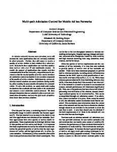
Fig. 2. Network topology after 50s of simulation

Figure 2 shows a typical network topology after 50s of simulation. It shows the geographic positions of the nodes with their respective transmission ranges. The dark nodes are the active nodes monitoring the network. The figure clearly shows that the border node detection scheme reliably identifies border nodes within the topology.

Fig. 3. Network topology after 500s of simulation

The figure above shows the topology again but after 500 seconds of simulation. The effect of the mobility model can be seen clearly. The node density is much higher in the center now, increasing the average neighbor count. The border node detection lost a slight bit of its accuracy. That can be

2 0

Fig. 4. Key parameters after 50s simulation

Figure 4 and 5 show the key parameters in more detail. They show the neighbor count which is the actual number of neighbors of each individual node in ascending order together with the locally calculated neighbor averages which is the network wide neighbor average calculated form the piggybacked data received by each individual node. The dashed horizontal line is the network wide neighbor average calculated employing global knowledge. The closer the local average of an individual node is to that line, the more reliable it can identify itself as a border node. If more nodes have a local average above that line, the overall system might generate a large number of active nodes. If the local average is in general calculated too low too few border nodes could be the result. That of course is also dependant on the way the threshold is calculated. From the figures one can see that at the beginning of the simulations we have a global average of 11 neighbors per node, whereas that average increases to 18 neighbors after 500 seconds. That translates into an increase of 63% in neighbor density. Figure 4 shows that the dynamically calculated neighbor average in general quite well reflects the real network wide average. Most of the nodes, though, have a local neighbor average slightly lower than the artificially extracted average. In the figure, the statistics of active nodes are shown in black (local average) and white (neighbor count) respectively. In figure 4 the values are all within the normal thresholds of the system i.e. activation threshold and neighborhood hysteresis.

Dynamic Border Node Detection Statistics after 500s 35

neighbor count local average

30

neighbor count (active node) local average (active node)

25 20

15 10

5 0

Fig. 5. Key parameters after 500s simulation

In figure 5 some of the values do not fully satisfy the system criteria due to the reasons already stated above. For example, the two rightmost border nodes in figure 5 should leave the active state next time they check their neighborhood. The reason why so many nodes have far less neighbors than the locally calculated threshold and are nonetheless not active is that they have a one hop neighbor which is already active. The important thing to notice is that the approach is stable. As can be seen from the figures 4 and 5, the neighbor average is not constant, but the system adapts to the changing environment and the border node count is not decreasing. The system is still fully functional. Per Node Neighbor Statisics 35

border node

Number of neighbors

30 25 20

threshold approach. The black marked data points are active nodes. What someone could do to increase the number of active nodes is to set the threshold relatively high. This way active nodes will be guaranteed, but their placement does not have to be optimal any more. With such a high threshold, the number of active nodes would not excessively grow in networks such as the one shown in figure 3. Nodes neighboring an active node would stay inactive and the density of the network would not allow the number of active node to grow unreasonably. We simulated the threshold approach in such networks with a threshold of 50, which is equal to the total number of nodes. This way every node would activate itself without having an active node in its radio range. The result was that only 12 nodes were activated leaving the number of active nodes at a reasonable number. The positions of the nodes within the network were left to chance and therefore the border node detection lost its relative determinism and usability. Even worse would be the effect in networks based on a short-range radio technology resulting in networks that are far less dense than the one shown in figure 3. The number of active nodes would further increase if the threshold is set to a high value. B. Centralized Network Partition Detection Figure 7 shows a typical centralized partition detection system structure. Clearly the server is the most vulnerable element of successful partition detection. For our simulations we chose the first node that activates itself to become the server. In a real network we would have to use a mechanism similar to a cluster head election phase used in hierarchical routing algorithms as already mentioned or a node initiating the application would serve as the beacon source (e.g. the game initiator).

15 threshold

10 5 0

Fig. 6. Neighbor statistics after 500s for the simple threshold approach

The simple threshold approach is not able to adapt to changing environments. The first problem is that the threshold has to be chosen very carefully. If it is too low, no or too few nodes become active which leads to a dysfunctional partition detection system. A second problem arises when the environment changes and nodes leave the system. This is of course only the case when the topology changes in a way that the average neighbor count increases like it does in the scenarios we tested. For the exact same movement traces the simple threshold approach always had less successfully detected border nodes at the end of simulation runs, when starting out with equal thresholds (see figure 6). Figure 6 shows the neighbor count of each individual node together with the threshold value (dashed line) for the simple

Fig. 7. Typical centralized partition detection system structure

For the first set of simulations we measured the amount of packets sent by the partition detection system averaged over 50 simulation runs without partitioning. The simulations lasted 500s and the results show the cost of operating the system (in terms of message exchanged) in the state that it should be in

most of the time (unpartitioned network). Centralized: Average number of packets exchanged during a 500s simulation run 10.2 1

2

buddy messages beacon messages broadcast messages notification messages fail messages 220.2

214.1

Fig. 8. Maintenance cost in number of messages sent

Figure 8 sums up the number of different messages exchanged. The parameters chosen in the simulation runs are the following. Every 15 seconds every node probed the neighborhood and then decided whether to change its state or not. The buddy sent a PING message every 5 seconds and the server sent a beacon message every 15 seconds to each of the border nodes. The figure does neither include the application data traffic nor the neighbor probes since they are equal in both approaches. As can be seen, the buddy traffic dominates the overall load generated by the system with nearly 50% (220.2) of the message total of 447.5 messages in average. These messages are in most cases one hop messages and therefore do not load the overall network. The other half of the messages generated mainly consist of beacon messages (214.1) which most likely are multi-hop messages loading the network more than the buddy messages do. The rest of the sent packets can be neglected except for the one broadcast message from the server at start-up. The main load of the partition detection system is carried by two nodes: the server and the server buddy. The server has to send all beacon messages and also 50% of the buddy packets (acknowledgements). Since the buddy changes during the simulation due to node mobility the rest of the buddy load is distributed over multiple nodes. The total traffic generated (447.5 messages) averaged over all nodes in the network would roughly translate into one packet sent per node every 55 seconds. In mobile gaming scenarios that amount of traffic would only be a fraction of the overall load generated by the application. The relation between partition detection inflicted load and load caused by the application is also highly dependent on the parameter set of the partition detection system. If an application needs to detect the partitioning relatively fast more packets have to be exchanged compared to a relatively slow detection process. In the simulations where we let nodes fail we concentrated on the server. The buddy always replaced the server and notified the other active nodes. The system could always

handle server failure. The only time it was not able to handle the failure and a false partition alarm was initiated was when both, server and buddy, failed simultaneously. Such a situation should be fairly rare, but to overcome this problem, an active node could elect more than one buddy node. Simultaneously failing border nodes could have an effect on the partition detection system only if by chance all border nodes in one partition failed after the partition occurred. The extra messages sent after a partition was detected are negligible compared to the messages sent throughout a simulation run. C. Distributed Network Partition Detection The distributed approach spans a mesh in the network topology (see figure 9). Every route from one active node to the other is sensitive to partition detection. The distributed approach of course generates much more traffic since much more beacon messages have to be exchanged and also every active node needs a buddy. The load generated can be seen in figure 10. The settings chosen are the same as for the distributed approach. Additionally, every active node should communicate with 3 other active nodes (temporarily less).

Fig. 9. Typical partnerships amongst nodes in the distributed approach

The average total message count sums up to an amount of 3121 messages. For the chosen parameter set that is roughly 7 times the amount of messages that have to be exchanged compared with the centralized approach. Again 50% or 1617 of those messages are one hop buddy messages. 904 beacon messages are exchanged amongst the active nodes. The individual load of a single active node, though, is far less than the server load in the centralized approach. Now also a significant amount of fail packets have to be sent. This kind of message includes notifications to active nodes if another active node changes its state. The other message types are

negligible except the request messages that in average sum up to 95.2 messages and describe the messages exchanged to build up a partnership between two active nodes. Distributed: Average number of packets exchanged during a 500s simulation run buddy messages

491.5

beacon messages broadcast messages

95.2

request messages

13.3

fail messages 1617

904

Fig. 10. Maintenance cost in number of messages sent

The simulations also showed that the distributed approach is much more resilient against node failure. The problem of simultaneously failing buddy and active nodes also persists here. If someone wanted to decrease the risk of such an unlikely event even more, multiple buddies would be the answer here as well.

Fig. 11: Partnerships amongst nodes during partitioning

The effectiveness of the distributed system is illustrated in figure 11. It shows the different partnerships that exist among the active nodes in the network. The separate partitions both contain 5 active nodes. 15 partnerships span the partitioned region. That means that 15 partnerships have to be destroyed in order to disrupt a successful partition detection. In this particular case it would mean to let nearly all active nodes fail simultaneously without giving the system time to recover. V. CONCLUSION & FUTURE WORK In this paper we have evaluated two different approaches to detect network partitioning. Both approaches are based on the

notion of border nodes and their successful identification. With both systems one is able to distinguish node failure from network partition, with both systems primarily differing in terms of resilience against failure and network load. To the best of our knowledge there are no partition detection mechanisms currently being employed in ad-hoc environments which explicitly select the best suited nodes and are also able to distinguish node failure from network partitioning. Our distributed approach is still extremely lightweight, of course depending on the temporal granularity of the detection mechanism, resilient, and efficient. Both our approaches have unique advantages. The centralized approach generates a by far lower message overhead compared to the distributed approach. It is in its structure much simpler, but burdens one single node far more than the rest of the nodes. The centralized approach also has some critical system states. For example during the time between server failure and the time when all active nodes registered at the new server the network is completely unmonitored. The same problem occurs during the time when a new server has to be elected in a separated partition. The server election phase itself could be a complex and costly task in terms of network load and system downtime. The distributed approach is far more resilient against node failure. Multiple partnerships make sure that a single or more failing nodes only reduce the monitored area of the affected nodes temporarily. That also has the effect that there is no downtime in that system except if a large number of nodes fail or an extremely unfortunate combination of nodes fail simultaneously. That also makes the system more stable against malicious nodes trying to disrupt the system. These positive properties of course come at a cost. The distributed approach loads the network far more than the centralized approach. In the future we plan to further evaluate the system. To reduce the load at the server, we are working on a scheme to allow the server to give up its role. This way the load is balanced amongst multiple nodes acting as a server at different times. We also want to evaluate whether the usage of routing state information instead of probing the network works with various routing algorithms such as AODV or DSR. The neighborhood probing at least could be substituted by such an approach, which would further reduce the network load. Since unicast messages also might cause controlled flooding of the network, depending on the routing protocol, we want to find the threshold where broadcasting messages is more efficient than using unicast messages. Although the separation of a buddy node from its corresponding active node during a network partition is a rare event, it might result in the network partition going undetected. Therfore, we want to evaluate a buddy election process based on average signal strength or another perhaps more suitable metric.

REFERENCES [1] [2] [3] [4] [5] [6]

T. Zippan, H. Ritter, A Survey of Gamers Expectations of Future Mobile Gaming Trends, Technical Report B04-04 Freie Universität Berlin, April 2004. The network simulator ns2. http://www.isi.edu/nsnam/ns/. Ö. Babaoglu, R. Davoli, A. Montresor, Group Communication in Partitionable Systems: Specification and Algorithms, IEEE Transactions on Software Engineering, 2001, vol. 27, no.4. M.-O. Killijian, R. Cunningham, R. Meier, L. Mazare, V. Cahill, Towards Group Communication for Mobile Participants, Workshop Transactions on Software Engineering, 2001, vol. 27, no.4. J. Bacon, K. Moody, J. Bates, R. Hayton, C. Ma, A. McNeil, O. Seidel, M. Spiteri. Generic Support for Distributed Applications. In IEEE Computer. 2000, vol. 33, no. 3. I. Keidar, D. Dolev. Totally Ordered Broadcast in the Face of Network Partitions. Dependable Network Computing, pages 51-75, D. Avresky Editor, Kluwer Academic Publication. January, 2000.

[7] [8] [9] [10] [11] [12]

[13]

Y. Amir, C. Nita-Rotaru, J. Stanton, G. Tsudik. Scaling Secure Group Communication Systems: Beyond Peer-to-Peer. DARPA Information Survivability Conference and Exposition. 2003. F. Kaashoek, A. Tanenbaum. Group Communication in the Amoeba Distributed Operating System. Symp. Reliable Distributed Systems. 1991 A. Ricciardi, K. Birman. Using Process Groups to Implement Failure Detection in Asynchronous Environments. Symp. Principles of Distributed Computing. 1998 Bluetooth. www.bluetooth.com. The working group for wireless LANs. http://grouper.ieee.org/groups/802/11/. T. Camp, J. Boleng, V. Davies. A Survey of Mobility Models for Ad Hoc Network Research. In Wireless Communication & Mobile Computing (WCMC): Special issue on Mobile Ad Hoc Networking: Research, Trends and Applications. 2002, vol. 2. M. Gerla, J. T.C. Tsai. Multicluster, Mobile, Multimedia Radio Network. In Wireless Networks, 1(3) 1995, pp. 255-265.