multiple, interdependent attacks on networked control systems. Under our framework, multiple .... networked control system design, they do not consider the dynamics of adversarial .... based on the following principles. First, the progress of the.
A Passivity-based Framework for Composing Attacks on Networked Control Systems Andrew Clark, Linda Bushnell, and Radha Poovendran Abstract— Networked control systems present an inviting target for adversaries seeking to attack physical infrastructure through cyber attacks alone. A diverse set of possible attacks, including node compromise, false data injection, malware propagation, and denial of service have been identified and studied in isolation. Currently, however, there is no framework for composing multiple attacks, mounted by one or more adversaries, and designing a system defense that guarantees stability and allows flexible performance. In this paper, we introduce a passivity framework for modeling and mitigating multiple, interdependent attacks on networked control systems. Under our framework, multiple adversaries are modeled as passive individual blocks, either in parallel or negative feedback interconnections depending on the interdependencies between the attacks, leading to an overall system that is passive and stabilizable. We present two case studies within this framework, namely joint node capture and malware propagation, as well as joint node capture and control channel jamming, and derive a stabilizing network response to the attacks. Our results are illustrated through a numerical study.
I. I NTRODUCTION Networked control systems are inviting targets for cyber attacks due to their prevalence in military and critical infrastructure applications. The goal of the attacks is to destabilize the plant or steer the plant to the adversary’s desired operating point, both of which will significantly degrade the performance of the system. Attacks are enabled by the fact that networked control systems consist of distributed components, many of which are physically unattended and patched infrequently [1], that communicate over an open wireless medium. The first step towards mitigating such attacks is to quantitatively model the combined actions of the adversaries and their impact on the targeted system. Attacks on control systems can be broadly classified into internal and external attacks. In an internal attack, an adversary compromises one or more nodes, extracts information from the nodes, and uses that information to masquerade as a valid network user. Examples of internal attacks include physical node capture [2] and malware propagation [3]. In an external attack, an adversary exploits the wireless communication medium to degrade the system performance through attacks such as denial of service [4], spoofing [5], and replay [6] attacks. Adversaries will further increase the damage to the system by mounting multiple attacks simultaneously, either individually or in cooperation with other adversaries. For example, by first compromising a set of network nodes, adversaries gain
inside information that enhances the impact of other attacks, such as frequency hopping sequences that can be exploited to increase the effectiveness of wireless jamming attacks. Currently, however, while methods have been proposed for mitigating individual attacks in both the network security and control-theoretic communities, there is no approach for composing multiple attacks and designing appropriate defense strategies. Such an approach, expressing both the attack and network defense in the control-theoretic language, would lead to guarantees in stability and performance of the system even in the presence of adversaries. In this paper, we present a passivity framework for modeling and mitigating multiple, composed attacks on networked control systems. In a passive system, energy injected into the system is dissipated internally over time; passivity is motivated by physical applications such as electric circuits and mechanical systems [7]. In the context of adversary modeling, our application of passivity is based on the observation that network resources used to thwart the attack, such as revoking and replacing compromised nodes, can be viewed as energy that is dissipated by an adversary who persistently and adaptively compromises the system. Furthermore, since parallel and negative feedback interconnections of passive systems are passive [8], passive models of individual attacks and network defenses can be composed while preserving the passivity property. We make the following specific contributions: •
•
•
A. Clark, L. Bushnell, and R. Poovendran are with the Department of Electrical Engineering, University of Washington, Seattle, WA, 91895, USA. Email: {awclark, lb2, rp3}@uw.edu
We introduce a passivity framework for modeling and composing attacks on networked control systems and for designing the appropriate system response. Our framework is used to prove the stability of the combined attack and response and characterize the steady-state of the system. We develop a passivity-based model of one or more adversaries simultaneously mounting a node capture attack, in which an adversary physically compromises unattended nodes, and a malware propagation attack, in which an adversary compromises nodes by introducing malicious code. We derive a passive dynamical model of each individual attack, and then prove that the composed adversary model is passive under the cases where (a) the attacks are executed independently, and (b) physically captured nodes are used to propagate malware into the system. We present a passive model of one or more adversaries mounting a physical node capture attack and using the captured nodes for intelligent jamming. We model the
impact of the jamming attack as an output of the node capture model, and prove the passivity of the overall adversary model. • For both case studies above, we derive a network response that causes the impact of the attack to converge to a steady-state value, which can be tuned by increasing the resources available for network defense. We derive the stable operating point as a function of the adversary capabilities and network defense parameters. • Our results are illustrated through a numerical study, in which we evaluate the effect of the network response parameters on the convergence and steady-state value of the system under attack. The paper is organized as follows. Section II reviews the related work. Section III gives background on passivity. Section IV describes our proposed passivity framework. Section V formulates and analyzes a passivity-based model of physical node capture and malware propagation attacks. Section VI discusses a passivity-based model of physical node capture and jamming attacks. Section VII presents numerical results. Section VIII concludes the paper. II. R ELATED W ORK Passivity methods have been used for modeling and analysis of a variety of network phenomena, including congestion control [9] and group coordination [10]. In [11], passivity techniques were used to design a stabilizing networked control system in the presence of time delays. In [12], a model of cyber-physical system integration was proposed that uses passivity to prove stability of networked control systems under uncertainties. While these existing works demonstrate the applicability of passivity techniques for networked control system design, they do not consider the dynamics of adversarial attacks on the system performance. Formulating models for specific, individual attacks in the control-theoretic language has been a subject of recent research interest. In [13], a linear dynamical model for physical node capture and cloning attacks by multiple adversaries was presented, and the optimal network response was studied using differential game theory. Dynamical models of malware propagation, including the optimal malware propagation strategy, were discussed in [3]. In [13] and [3], however, the proposed approaches are valid for attacks of a single type but do not consider composition of multiple, interrelated adversary models. III. M ODELS
AND
BACKGROUND
In this section, we first give the network model and describe the adversary models used in Sections V and VI. We then give relevant background on passivity theory. A. System Model We consider a network consisting of N nodes. The nodes are physically unattended and operated over an extended period of time. The nodes communicate over a shared wireless medium in order to coordinate their control action, as well as monitor other nodes for suspicious behavior.
A revocation mechanism is assumed to exist for removing potentially compromised nodes from the system. B. Adversary Model – Joint Node Capture and Malware Propagation In a node capture attack, an adversary physically tampers with an unsupervised device. By doing so, the adversary gains control over all the device’s hardware and software. In a malware propagation attack, the adversary uses compromised nodes to introduce malicious code into the network. A node that receives and installs the malicious code is compromised by the adversary, and can be used to introduce new malware into the system. Nodes that are compromised, either through node capture or malware propagation, can be used to mount secondary attacks such as eavesdropping, packet injection or control channel jamming. Physical node capture attacks are typically identified by observing malicious behaviors from the compromised nodes. For example, a node capture attack may identify insiders mounting intelligent jamming attacks [4]. Malware can be detected either through anomalous node behavior, or by comparing suspicious code with known examples of malware. Once a compromised node has been detected, it can either be quarantined, cleaned, and returned to the network, or removed and replaced. C. Adversary Model – Joint Node Capture and Control Channel Jamming In a jamming attack, an adversary broadcasts an interfering signal in the vicinity of a valid receiver in order to prevent the receiver from correctly decoding packets. Jamming of control packets, which contain protocol data used by nodes to provide network services, can be especially damaging to network connectivity and performance. In order to prevent control channel jamming, network nodes may alternate between multiple frequencies at different time slots; let Fi be the set of frequencies held by node i. An adversary who does not know the frequency used at a given time slot will not be able to effectively jam the control messages. An adversary who has compromised one or more nodes, however, through a node capture attack can extract the sequence of frequency hops from the captured nodes and jam those channels. Letting C denote the set of compromised nodes, the set of jammed channels is equal to J = ∪i∈C Fi . Defenses against control channel jamming are based on identifying and removing nodes whose channels are being jammed. One approach is to identify the set of nodes i satisfying Fi ⊆ J and revoke those nodes. This approach involves an inherent trade-off between thwarting the jamming attack by revoking compromised nodes, and the cost of falsely revoking valid nodes [14]. D. Background on Passivity Theory We consider a dynamical system with state-space X ⊆ Rn and time-varying state x(t) ∈ X . The input u(t) belongs to set U ⊆ Rm , while the output y(t) lies in set Y ⊆ Rm . The
system is represented by the state-space dynamical model Σ, defined by � x(t) ˙ = f (x(t), u(t)) (Σ) (1) y(t) = g(x(t), u(t)) where the functions f and g are continuously differentiable. The passivity property is defined as follows. Definition 1 (Passivity [7]): The system (Σ) of (1) is passive if there exists a constant γ such that Z t y T (s)u(s) ds ≥ γ 0
for all functions u and all t ≥ 0. More generally, a system is dissipative with supply rate α : U × Y → R if there exists a function V : R → R such that Z t α(u(s), y(s)) ds. (2) V (t) ≤ V (0) + 0
The supply corresponds to the rate at which energy is supplied to the system by the input/output processes. A passive system is dissipative with supply rate α(u(t), y(t)) = u(t)T y(t). The following lemma gives an equivalent definition of passivity. Lemma 1 ( [7]): Consider the system (Σ). Assume that there exists a nonnegative and continuously differentiable function V and a measurable function d such that Rt d(s) ds ≥ 0 for all t ≥ 0. If V˙ (t) ≤ u(t)T y(t) − d(t) for 0 all t ≥ 0 and all functions u, then the system (Σ) is passive. If V˙ (t) ≤ α(u(t), y(t)) − d(t), then the system is dissipative with supply rate α. The function V (t) in Lemma 1 can be interpreted as the amount of energy stored in the system at time t. The lemma implies that, if a system is passive, then the rate at which energy exits the system is less than the input times the output. A key advantage of the passivity framework is that interconnections between passive systems are passive, as described by the following two lemmas. Lemma 2 ( [9]): A negative feedback interconnection between two passive systems is stable in the sense of Lyapunov. Lemma 3 ( [9]): A parallel interconnection between two passive systems is passive. The following result gives a necessary and sufficient condition for passivity of a class of nonlinear systems with affine input. Lemma 4 (Nonlinear KYP Lemma [7]): Define a special case of (Σ), denoted (Σ′ ), as follows: � x(t) ˙ = f (x(t)) + g(x(t))u(t) (Σ′ ) (3) y(t) = h(x(t))
The system is passive for S(x) ≥ 0 and strictly passive if S(x) > 0. (ii) There exists a continuously differentiable nonnegative function V : X → R with V (0) = 0 such that ∂V (x) ∂x f (x) = −S(x) (4) ∂V (x) T g(x) = h (x) ∂x The following lemma gives an approach for designing a stabilizing controller for a passive system. The definition of zero-state detectability is needed as a preliminary. Definition 2 ( [7]): The nonlinear system (3) is zero-state detectable if, for any x(t), u(t) = 0, h(x(t)) = 0, ∀t ≥ 0 ⇒ lim x(t) → 0. t→∞ Lemma 5 ( [7]): Suppose that the system (3) is passive and zero-state detectable. Let φ(y) be any smooth function such that φ(0) = 0 and y T φ(y) > 0, ∀y 6= 0. Assume that the storage function V (x) > 0 is proper, i.e., the set V −1 ([0, τ ]) is compact for each τ > 0. Then the control law u = −φ(y) achieves global asymptotic stability of x = 0. IV. P ROPOSED PASSIVITY F RAMEWORK Our proposed passivity framework for modeling and composing adversary models and network defenses is described in this section. The framework is illustrated in Figure 1.
Fig. 1. Block diagram illustrating the dynamical modeling of the adversary and network response. The response consists of two blocks, a proactive component that detects suspicious nodes and a reactive component that responds to increases in adversary activity. When the adversary model is passive, the network response can be designed to steer the state of the system to a desired steady-state value.
The first block (Figure 1, top block) consists of a dynamical systems representation of one or more adversaries’ actions over time. Our dynamical modeling approach is based on the following principles. First, the progress of the attack is described by a time-varying state, representing the extent to which the network has been compromised. Second, an intelligent and adaptive adversary will update its attack strategy based on its current state and the response of the where f , g, and h are smooth functions and u and y denote network defender. Third, the impact of the attack can be the input and output of the system, respectively. Then the viewed as an output, which the network can use to make a partial observation of the attack state. following are equivalent: Our motivation for studying the passivity of the adversary (i) There exists a function V (x) ≥ 0, V (0) = 0 and a model is to consider the network response to the attack, function S(x) ≥ 0 such that for all t ≥ 0, which may include removing nodes or refreshing keying Z t Z t material, as an input that introduces energy into the system. S(x(s)) ds. y T (s)u(s) ds− V (x(t))−V (x(0)) = This input is then dissipated by the adversary’s actions, 0 0
drawing the system to a low-energy state representing a fully compromised network. The bottom two blocks of Figure 1 consist of a dynamical systems representation of the network response to the attack. Similar to the adversary model, the network response model considers a network response state that evolves over time in response to the observed impact of the attack and the current network state. The network response considered in this paper has two subcomponents. The first subcomponent consists of a defense mechanism that monitors possible adversary actions at all times and changes the network state if suspicious behaviors are detected. This subcomponent can be viewed as proactive, since it operates even in the absence of adversary activity. The second subcomponent consists of defense mechanisms that only activate in response to an increase in adversary activity. This reactive subcomponent responds to changes in the adversary’s behavior by expending additional resources to steer the system to its desired state. The main goal of this modeling approach is to prove that the combined system, consisting of the adversary and the network response, converges to a stable equilibrium point. The network response can then be chosen to achieve a desired steady-state, subject to constraints or costs on the resources available for the response. V. M ODELING AND M ITIGATING N ODE C APTURE M ALWARE ATTACKS
AND
This section applies our proposed framework to modeling one or more adversaries who execute two simultaneous attacks, one based on physical node capture and the other on malware propagation. We present a dynamical model of the attacks, which we show to be passive. We then consider two interconnections between node capture and malware attacks. In the first case, the node capture and malware attacks are independent and are modeled as a passive interconnection. In the second case, nodes that are physically captured are used to propagate malware. We then introduce a dynamical model for the network response, which we show to be passive as well. Based on the passivity proofs, we analyze the number of compromised nodes in the system in steady-state. A. Dynamical Models of Node Capture and Malware Propagation A dynamical model for the node capture attack is as follows. Let x1 (t) denote the fraction of nodes that have been captured, y1 (t) denote the output of the node compromise process, and w1 (t) denote the rate at which captured nodes are removed at time t. Then the dynamical model of node capture considered in this work is given by � x˙ 1 (t) = λ(1 − x1 (t)) − w1 (t) (5) y1 (t) = x1 (t) where λ ∈ [0, 1] is the capture rate. This model, which is discussed further in [13], is based on the fact that, as the fraction of captured nodes increases, the rate at which an adversary can locate valid nodes to capture
decreases. The passivity of the model (5) is described by the following proposition. Proposition 1: The model (5) is passive with input u1 (t) = −w1 (t) and output z1 (t) = y1 (t) − 1. Proof: Define the storage function V1 (t) = 12 (1 − x1 (t))2 . Then we have V˙ 1 (t) = −(1 − x1 (t))x˙ 1 (t) = −(1 − x1 (t))(λ(1 − x1 (t)) + u1 (t)) = −λ(1 − x1 (t))2 + u1 (t)(x1 (t) − 1) = −λ(1 − x1 (t))2 + u1 (t)z1 (t), establishing passivity by Lemma 1. We study malware propagation using an epidemic model, in which each node that has been compromised by malware attempts to infect the remaining nodes. In this model, which has been considered in [3], x2 (t) is equal to the fraction of compromised nodes, y2 (t) is equal to the fraction of compromised nodes that are detected, and w2 (t) is equal to the fraction of compromised nodes that are detected and revoked. We assume that x2 (0) ∈ [0, 1]. The model is given by � x˙ 2 (t) = νx2 (t)(1 − x2 (t)) − w2 (t) (6) y2 (t) = x2 (t) where ν ∈ [0, 1] is the propagation rate. We require that w2 (t) satisfy the following properties. First, w2 (t) ∈ [0, 1]. Second, w2 (t) = 0 when x2 (t) = 0 (otherwise it would imply that compromised nodes are revoked when there are no compromised nodes). The following lemma gives necessary properties to prove passivity of (6) under these assumptions. Lemma 6: Under the model (6) and the assumptions given above, x2 (t) ∈ [0, 1] for all t ≥ 0. A proof is given in the appendix. The following proposition implies that the malware propagation model (6) is a passive system as well. Proposition 2: The malware propagation model (6) is passive with input u2 (t) = −w2 (t) and output z2 (t) = y2 (t)−1. Proof: Define the storage function V2 (t) = 12 (1 − x2 (t))2 . We then have V˙ 2 (t) = −(1 − x2 (t))x˙ 2 (t) = −(1 − x2 (t))(νx2 (t)(1 − x2 (t)) + u2 (t)) = −νx2 (t)(1 − x2 (t))2 + u2 (t)z2 (t).
(7)
By Lemma 6, the first term of (7) is strictly negative, and hence (6) is a passive system by Lemma 1. B. Composing Node Capture and Malware Propagation Models In this section, the passivity of two models of interconnected node capture and malware propagation attacks are considered. In the first model, the node capture and malware attacks are mounted independently, leading to a parallel interconnection. In the second model, physically captured nodes are used to mount the malware propagation attack. The following proposition describes the passivity of a composed
system, consisting of one or more adversaries mounting independent node capture and malware propagation attacks. Proposition 3: The dynamical model x˙ 1 (t) = λ(1 − x1 (t)) − w1 (t) x˙ 2 (t) = νx2 (t)(1 − x2 (t)) − w2 (t) (8) y1 (t) = x1 (t), y2 (t) = x2 (t)
is passive from (u1 (t), u2 (t)) = (−w1 (t), −w2 (t)) to (x1 (t) − 1, x2 (t) − 1). Proof: By Propositions 1 and 2, system (8) is a parallel interconnection of passive systems, and hence is passive by Lemma 3.
Fig. 2. Block diagram of the dynamical model in (8), showing parallel node capture (with state x1 (t)) and malware propagation (with state x2 (t)) attacks and the network response (w1 (t), w2 (t)).
The joint model described by (8) is illustrated in Figure 2. We now consider a sophisticated model of joint node capture and malware attacks, in which nodes that are physically captured are used to propagate malware, within the passivity framework as follows. Define a joint node capture and malware propagation model by x˙ 1 (t) = λ(1 − x1 (t) − x2 (t)) − w1 (t) x˙ 2 (t) = ν(x1 (t) + x2 (t))(1 − x1 (t) − x2 (t)) − w2 (t) y1 (t) = x1 (t), y2 (t) = x2 (t) (9) Under this model, nodes that have been already compromised by malware are not physically captured as well. Furthermore, physically captured nodes are used alongside nodes compromised by malware to propagate the malware code. The following theorem describes the passivity of (9). Theorem 1: The joint node capture and malware propagation model (9) is dissipative with input u(t) = (u1 (t), u2 (t)) = (−w1 (t), −w2 (t)), output y(t) = (x1 (t), x2 (t) − 1), and storage function τ (u, y) = u11T y, where 1 is the vector of all ones. Proof: Define V (t) = 12 (1 − x1 (t) − x2 (t))2 . Then V˙ (t) = −(1 − x1 (t) − x2 (t))(x˙ 1 (t) + x˙ 2 (t)) = −(1 − x1 (t) − x2 (t))(λ(1 − x1 (t) − x2 (t)) + u1 (t) +ν(x1 (t) + x2 (t))(1 − x1 (t) − x2 (t)) + u2 (t)) < u1 (t)(x1 (t) + x2 (t) − 1) + u2 (t)(x1 (t) + x2 (t) − 1) = u(t)T 11T y(t) as desired.
C. Dynamical Model of Network Response The network response consists of identifying and revoking nodes that have been compromised. In this section, we treat the network response to the node capture and malware propagation attacks separately, and then develop a combined response model for the parallel interconnection (8), leaving the response to (9) for future work. We first consider the network response to the physical node capture attack. 1) Network response to node capture: In the dynamical model, we divide the network response into two components. First, the network runs a detection process that identifies a node as compromised within an interval of length dt with probability µ1 dt. Second, there is a component of the network response, given by v1 (t), that varies the revocation rate in response to increases in adversarial activity. It is assumed that µ1 and v1 (t) can take arbitrary values in [0, ∞); this corresponds to an assumption that the network can always increase the detection rate by expending additional resources (trade-offs between this resource expenditure and the security of the system are explored further in Section VII). As a result, the dynamics of the physical node capture attack are given as � x˙ 1 (t) = λ(1 − x1 (t)) − µ1 x1 (t) − v1 (t) (10) y1 (t) = x1 (t) As a preliminary to choosing the dynamics of v1 (t), properties of (10) are needed. First, observe that (10) has λ when v1 (t) ≡ 0. Letting an equilibrium point at x∗1 = λ+µ 1 ∗ x ˆ1 (t) = x1 (t) − x1 , the dynamics (10) can be rewritten as � x ˆ˙ 1 (t) = −(λ + µ1 )ˆ x1 (t) − v1 (t) (11) yˆ1 (t) = x ˆ1 (t) which has an equilibrium point at xˆ1 = 0. The following proposition describes the passivity properties of (11). Proposition 4: The dynamical model (11) is zero-state detectable and passive with input (−v1 (t)) and output yˆ1 (t). Proof: Zero-state detectability follows from the fact that yˆ1 (t) = x ˆ1 (t), and hence yˆ1 (t) ≡ 0 if and only if x ˆ1 (t) ≡ 0. Define Vˆ1 (t) = 12 xˆ1 (t)2 . Then we have ˙ Vˆ1 (t) = x ˆ1 (t)x ˆ˙ 1 (t) =x ˆ1 (t)(−(λ + µ1 )ˆ x1 (t) − v1 (t)) = −(λ + µ1 )ˆ x1 (t)2 − xˆ1 (t)v1 (t) ≤x ˆ1 (t)(−v1 (t)) with equality iff x ˆ1 (t) = 0, as desired. We define the revocation strategy v1 (t) = β1 (x1 (t) − x∗1 ). The following proposition defines the stability and convergence properties of the system (10) with this choice of v1 (t). Proposition 5: Let v1 (t) = β1 (x1 (t) − x∗1 ). Then the λ as a globally asymptotically dynamics (10) has x∗1 = λ+µ 1 stable equilibrium point. Proof: The proof follows from Lemma 5 along with Proposition 4. Remark 1: Lemma 5 implies that a broader class of network responses v1 (t) will result in global asymptotic stability of (10). These alternative strategies may result in different convergence rates and costs for the network.
2) Network response to malware propagation: As in the case of physical node capture, we introduce a proactive detection process, which detects and revokes a compromised node during a time interval of length dt with probability µ2 dt, as well as a reactive process v2 (t). This leads to the augmented dynamical model � x˙ 2 (t) = νx2 (t)(1 − x2 (t)) − µ2 x2 (t) − v2 (t) (12) y2 (t) = x2 (t) By examination, the dynamical model (12) has two fixed points when the input v2 (t) ≡ 0, namely x2 = 0 and x2 = (1 − µν2 ). The fixed point that is achieved by the system depends on the values of µ2 and ν. The passivity of (12) can be shown for certain values of the parameters µ2 and ν. Proposition 6: Suppose that µ2 > ν. Then the dynamics (12) are passive and zero state detectable from the input −v2 (t) to the output y2 (t). Proof: Define Vˆ2 (t) = 12 x2 (t)2 . Then differentiating with respect to t yields ˙ Vˆ2 (t) = x2 (t)(νx2 (t)(1 − x2 (t)) − µ2 x2 (t) − v2 (t)) = x2 (t)2 (ν − νx2 (t) − µ2 ) − v2 (t)x2 (t), and hence the system is passive if ν − νx2 (t) − µ2 < 0 for all x2 (t) ∈ [0, 1]. The condition ν < µ2 implies that this is indeed the case. Proposition 6 motivates a controller v2 (t) for (12), given by v2 (t) = β2 (y2 (t)). The following proposition describes the stability of the overall system. Proposition 7: The dynamics (12) with v2 (t) = β2 y2 (t) are globally asymptotically stable at x2 = 0 if µ2 > ν. Proof: By Lemma 5 and Proposition 6, the controller v2 (t) = β2 (y2 (t)) drives the state x2 (t) of (12) to 0. 3) Response to joint node capture and malware propagation: In responding to the composed dynamics (8), we leverage the fact that a parallel interconnection of passive systems is passive. Hence, by Propositions 4 and 6, as well as Lemma 3, the joint dynamics ˆ˙ 1 (t) = λ(1 − x ˆ1 (t) − x∗1 ) − µ1 (ˆ x1 (t) + x∗1 ) − v1 (t) x x˙ (t) = νx2 (t)(1 − x2 (t)) − µ2 x2 (t) − v2 (t) 2 y1 (t) = xˆ1 (t), y2 (t) = x2 (t) (13) are passive and zero-state detectable from input (−v1 (t), −v2 (t)) to output (y1 (t), y2 (t)). Hence a controller given by v1 (t) = β1 (y1 (t) − x∗1 ), v2 (t) = β2 y2 (t) will achieve global asymptotic stability of the system. VI. M ODELING AND M ITIGATING N ODE C APTURE I NSIDER JAMMING ATTACKS
AND
In this section, we describe a case study of an attack in which one or more adversaries physically capture a set of nodes, and then use the captured nodes to mount a control channel jamming attack. We describe dynamical models and passivity analysis of the jamming attack and the network’s defense against the composed attack.
A. Dynamical Model of Insider Jamming The impact of the insider jamming attack is quantified by the fraction of channels that are jammed at time t, which we denote y(t). We model y(t) as an output of the node capture process, defined by x(t) ˙ = λ(1 − x(t)) − w(t), where w(t) is the rate at which compromised nodes are identified and revoked. The value of y(t) is therefore equal to the fraction of channels that can be jammed by an adversary who has captured x(t) nodes. The derivation of y(t) is given by the following lemma. Lemma 7: Suppose that each node has access to each control channel with probability p, and does not have access with probability q = 1 − p. Let qˆ = q N , where N is the total number of nodes. Then the fraction of channels y(t) that can be jammed by an adversary who has compromised x(t) nodes is equal to y(t) = 1 − qˆx(t) . A proof is contained in the appendix. The dynamical model of insider jamming can therefore be written as � x(t) ˙ = λ(1 − x(t)) − w(t) (14) y(t) = 1 − qˆx(t) . The passivity of the model (14) is given by the following proposition. Proposition 8: The dynamical model (14) is passive from input u(t) = −w(t) to output z(t) = y(t) − 1. Proof: Let a = − ln qˆ, so that a > 0. Define V (t) = 1 −ax(t) e . The fact that y(t) − 1 = −e−ax(t) implies a V˙ (t) = −e−ax(t) x(t) ˙ = −e−ax(t) (λ(1 − x(t))) − w(t)) = −e−ax(t) (λ(1 − x(t))) − w(t)(y(t) − 1) = −e−ax(t) (λ(1 − x(t))) + u(t)z(t).
(15)
The first term of (15) is nonpositive since x(t) ∈ [0, 1], giving the desired result. B. Dynamical Model of Network Response In this section, we describe a dynamical model of the network response to the combined node capture and control channel jamming attack, given in (14). As in Section V-C, the response consists of two components: a proactive detection strategy that revokes a fraction µ of compromised nodes per unit time, and a reactive response v(t) that increases the convergence speed of the fraction of jammed channels to the desired steady-state value, y ∗ . Let x∗ = − a1 ln (1 − y ∗ ), equal to the fraction of compromised nodes resulting in y ∗ jammed channels. Define the output of the system to be yˆ(t) = y(t) − y ∗ . The augmented network dynamics, including the proactive detection mechanism, are given by � x(t) ˙ = λ(1 − x(t)) − µx(t) − v(t) ∗ ∗ yˆ(t) = (1 − e−ax(t) ) − y ∗ = e−ax (1 − e−a(x(t)−x ) ) (16) Setting xˆ(t) = x(t) − x∗ results in the equivalent dynamics � x ˆ˙ (t) = −(λ + µ)ˆ x(t) − v(t) ∗ (17) yˆ(t) = e−ax (1 − e−aˆx(t) )
Effect of parameters on number of jammed channels 0.4
Effect of detection parameters on cost to system 5.7
0.35 Fraction of jammed channels
5.6
Cost to system
5.5 5.4 5.3 5.2 β=1 β=2 β=3
5.1 5 4.9 0.5
0.25
0.2
0.15
0.1
0.05
1
Revocation rate µ
1.5
β=1, µ=4 β=1, µ=10 β=3, µ=4 β=3, µ=10
0.3
2
0
2
4
6
8
10
Time
(a)
(b)
Fig. 3. Numerical evaluation of our proposed passivity framework. (a) Cost to the system resulting from the activity of captured nodes and the cost of detection and revocation, with λ = ν = 1. The cost reaches a local minimum at µ1 = µ2 = µ = 1 for all values of β1 = β2 = β. (b) The fraction of jammed channels as a function of time. The fraction of jammed channels is determined by µ, while the rate of convergence is determined by β.
The network response is based on the following proposition. Proposition 9: The system (17) is passive and zero-state detectable. Proof: Passivity is verified using the nonlinear KYP lemma (Lemma 4). The second condition of (4) implies that the system is passive only if there exists V satisfying ∂V = yˆ(t). ∂x ˆ The solution to (18) satisfying V (0) = 0 is given by
(18)
∗ 1 V (t) = e−ax (ˆ x(t) − (1 − e−aˆx(t) )). a It remains to verify the first condition of (4). We have ∗ ∂V = e−ax (1 − e−aˆx(t) )(−(λ + µ))ˆ x(t). (19) ∂x ˆ If x ˆ(t) < 0, then the first term of (19) is negative and the second term is positive. On the other hand, if xˆ(t) > 0, then the first term is positive and the second term is negative. Thus ∂V ∂x ˆ < 0, establishing passivity of (17) by Lemma 4. To prove zero-state detectability, note that yˆ(t) ≡ 0 implies that e−aˆx(t) ≡ 1, which implies that x ˆ(t) ≡ 0. Proposition 9 leads to the following network defense strategy. Let v(t), the rate at which nodes are revoked, be given by v(t) = β yˆ(t) for β ∈ [0, 1]. The following proposition establishes the stability of the system under this defense. Proposition 10: The system (17) is globally asymptotically stable with equilibrium x∗ under the network response v(t) = β yˆ(t). Proof: Follows from Lemma 5 and Proposition 9.
VII. N UMERICAL S TUDIES In order to illustrate our approach, we perform numerical studies using Matlab. We considered a network under node capture and malware attack with parameters λ = ν = 1. The revocation rate µ = µ1 = µ2 varies from 0.5 to 2, while the
rate β = β1 = β2 varies from 1 to 3. In the case of control channel jamming, the parameter a is set equal to 1. The goals of the simulation are (i) to determine the effect of the parameters µ and β on the steady-state value of the system and (ii) to empirically observe the stability and convergence properties. Question (i) is addressed for the system (8) in Figure 3(a). We compute the cost to the system of both compromised node activity and detection and revocation, which we define as Z τ x(t)T x(t) + u(t)T u(t) dt C= 0
with τ = 10, x(t) = (x1 (t), x2 (t)), and u(t) = (−w1 (t), −w2 (t)). We observe that the cost reaches a minimum at µ = 1, implying that for larger values of µ the resource cost of detecting compromised nodes exceeded the security benefit. We further observe that a lower β value results in lower overall cost. This suggests a tradeoff between stability and performance; while a low β value may reduce the cost, the guarantees of Proposition 4 would no longer hold with β = 0. Figure 3(b) addresses question (ii) for the system (14). We observe that the number of jammed channels in steady-state is determined by µ. The parameter β determines the rate at which the dynamics converge to the steady-state value. VIII. C ONCLUSION We considered the problem of modeling one or more adversaries mounting multiple insider and external attacks on a networked control system. We introduced a passivity framework for composing dynamical models representing the attacks and the network response. Two case studies were analyzed within this framework. First, a dynamical model of one or more adversaries compromising nodes through physical node capture and malware propagation was formulated. The passivity of a parallel interconnection, representing two independent attacks, was proved, followed by the passivity of a more general interdependence between the attacks. Second,
a dynamical model of one or more adversaries mounting a combined node capture and control channel jamming attack was presented. The jamming attack was modeled as the nonlinear output of the physical node capture process. For each model, we derived a stabilizing controller that achieves a globally asymptotic equilibrium, which can be tuned by the network in order to satisfy a desired costbenefit trade-off. The stabilizing controller can be interpreted as a defense strategy with two components: (a) a proactive component, which constantly monitors the network and identifies suspicious nodes, and (b) a reactive component, which responds to deviations from the desired state by increasing the resources devoted to network monitoring and compromised node revocation. A numerical analysis was used to study the cost to the network for different values of the defense parameters, and suggests that there exist finite, optimal parameters for network defense. Future work will focus on identifying general composition rules that can be applied to a broad class of attacks, including Byzantine attacks in which an adversary, after compromising a set of nodes, uses them to disrupt network protocols such as routing. We will also explore the space of defense strategies that satisfy stability within our framework, as well as how to incorporate uncertainty into the adversary model and adjust the network response accordingly. R EFERENCES [1] D. Beresford, “Exploiting Siemens Simatic S7 PLCs,” Black Hat USA, 2011. [2] P. Tague and R. Poovendran, “Modeling adaptive node capture attacks in multi-hop wireless networks,” Ad Hoc Networks, vol. 5, no. 6, pp. 801–814, 2007. [3] M. Khouzani, S. Sarkar, and E. Altman, “Maximum damage malware attack in mobile wireless networks,” Proceedings of the IEEE Infocom, pp. 1–9, 2010. [4] A. Chan, X. Liu, G. Noubir, and B. Thapa, “Broadcast control channel jamming: Resilience and identification of traitors,” Proceedings of the IEEE International Symposium on Information Theory (ISIT), pp. 2496–2500, 2007. [5] Y. Liu, P. Ning, and M. Reiter, “False data injection attacks against state estimation in electric power grids,” ACM Transactions on Information and System Security (TISSEC), vol. 14, no. 1, pp. 1–33, 2011. [6] Y. Mo and B. Sinopoli, “Secure control against replay attacks,” 47th Annual Allerton Conference on Communication, Control, and Computing, pp. 911–918, 2009. [7] R. Lozano, B. Brogliato, O. Egeland, and B. Maschke, Dissipative Systems Analysis and Control: Theory and Applications. Springer London, 2000. [8] J. Willems, “Dissipative dynamical systems Part I: General theory,” Archive for Rational Mechanics and Analysis, vol. 45, no. 5, pp. 321– 351, 1972. [9] J. Wen and M. Arcak, “A unifying passivity framework for network flow control,” IEEE Transactions on Automatic Control, vol. 49, no. 2, pp. 162–174, 2004. [10] M. Arcak, “Passivity as a design tool for group coordination,” IEEE Transactions on Automatic Control, vol. 52, no. 8, pp. 1380–1390, 2007. [11] H. Yu and P. Antsaklis, “Event-triggered output feedback control for networked control systems using passivity: Time-varying network induced delays,” Proceedings of the 50th IEEE Conference on Decision and Control and European Control Conference (CDC-ECC), pp. 205– 210, 2011. [12] J. Sztipanovits, X. Koutsoukos, G. Karsai, N. Kottenstette, P. Antsaklis, V. Gupta, B. Goodwine, J. Baras, and S. Wang, “Toward a science of cyber–physical system integration,” Proceedings of the IEEE, vol. 100, no. 1, pp. 29–44, 2012.
[13] Q. Zhu, L. Bushnell, and T. Bas¸ar, “Game-theoretic analysis of node capture and cloning attack with multiple attackers in wireless sensor networks,” Proceedings of the 51st IEEE Conference on Decision and Control (CDC), 2012. [14] P. Tague, M. Li, and R. Poovendran, “Mitigation of control channel jamming under node capture attacks,” IEEE Transactions on Mobile Computing, vol. 8, no. 9, pp. 1221 –1234, 2009.
A PPENDIX In this appendix, proofs of Lemmas 6 and 7 are given. Proof: [Proof of Lemma 6] First, suppose that x2 (t) > 1. Let S = {s ∈ (0, t) : x2 (s) = 1}. Since x2 (0) ∈ [0, 1] and x2 (t) is continuous, S is nonempty; furthermore, all elements of S are bounded by t. Let s∗ = sup S. Then x˙ 2 (s∗ ) = νx2 (s∗ )(1 − x2 (s∗ )) − w2 (s∗ ) = ν(1)(0) = w2 (s∗ ) ≤ 0, using the fact that w2 (s∗ ) ∈ [0, 1]. Thus there exists ǫ > 0 such that x2 (t′ ) ≤ 1 for all t′ ∈ [0, ǫ), and so by continuity of x2 (t) there exists s′ ∈ [s∗ + ǫ, t) ∩ S. This, however, contradicts the assumption that s∗ = sup S, thereby establishing x2 (t) ≤ 1. Now, suppose that x2 (t) < 0. Then there exists s ∈ (0, t) with x2 (s) = 0, and x˙ 2 (s) = νx2 (s)(1 − x2 (s)) − w2 (s) = 0. Hence x2 (t′ ) = 0 for all t′ ∈ [s, ∞), contradicting the assumption that x2 (t) < 0. Proof: [Proof of Lemma 7] The fraction y(t) is equal to the probability that a given channel is jammed. Let J denote the event that a channel is jammed, and let J c denote the complementary event. Let N denote the set of nodes that have access to that channel. Then we have y(t) = P r(J) = 1 − P r(J c ) = 1 − P r (∩i∈N i ∈ / C) x(t)N
=1−
Y
P r(i ∈ / N)
i=1 x(t)N
=1−q as desired.
= 1 − qˆx(t)