A Path-Optimal GAC Algorithm for Table Constraints - CiteSeerX

A Path-Optimal GAC Algorithm for Table Constraints Christophe Lecoutre1 and Chavalit Likitvivatanavong and Roland H. C. Yap2 Abstract. Filtering by Generalized Arc Consistency (GAC) is a fundamental technique in Constraint Programming. Recent advances in GAC algorithms for extensional constraints rely on direct manipulation of tables during search. Simple Tabular Reduction (STR), which systematically removes invalid tuples from tables, has been shown to be a simple yet efficient approach. STR2, a refinement of STR, is considered to be among the best filtering algorithms for positive table constraints. In this paper, we introduce a new GAC algorithm called STR3 that is specifically designed to enforce GAC during search. STR3 can completely avoid unnecessary traversal of tables, making it optimal along any path of the search tree. Our experiments show that STR3 is much faster than STR2 when the average size of the tables is not reduced drastically during search.

1

Introduction

Constraint propagation, which consists in calling iteratively filtering algorithms associated with constraints, is one of the most attractive features of Constraint Programming (CP). The various levels of possible filtering are typically described by properties of constraint networks called consistencies. Generalized Arc Consistency (GAC), which corresponds to the highest filtering level of variable domains when constraints are considered independently, is such a property. GAC is one very important lever to solve efficiently Constraint Satisfaction Problems (CSPs) because it identifies many more inconsistent values than limited consistency forms (e.g., those defined on domain bounds or dependent on the number of assigned variables), reducing search space considerably as a consequence. Table constraints are defined in extension by explicitly listing all permitted combinations of values (positive tables) or all forbidden ones (negative tables). Table constraints naturally arise in many application areas such as configuration and databases, and besides they can be viewed as a universal mechanism for representing any constraints. Classical filtering algorithms (e.g. [3, 4, 9, 10]) generally do not alter table constraints during backtrack search. Recent developments, however, suggested handling tables directly, which leads to faster algorithms [8, 13]. Alternatively, specially-constructed intermediate structures such as tries [7] or Multi-valued Decision Diagrams (MDDs) [6] have been proposed. In any case, the search space gets smaller as the tables or their equivalent structures are reduced. Most GAC algorithms follow the same pattern: a value is proved to be consistent by producing a valid tuple containing that value (in the case of positive table constraints) or by producing evidence from auxiliary structures (a path from top to bottom in the case of MDDs). This is usually performed by traversing these structures and running tests on each chunk. Reducing the amount of traversal has long been the focus of a many works resulting in many optimization techniques. 1 2

CRIL-CNRS, UMR 8188, Universit´e d’artois, France, [email protected] School of Computing, National University of Singapore, Republic of Singapore, [email protected], [email protected]

Simple Tabular Reduction (STR) and its improvements [8, 13] fall into this category and have been shown to be among the best GAC algorithms for positive table constraints. The main idea of STR is to remove invalid tuples systematically from tables immediately. In this paper, we introduce a new GAC algorithm called STR3. It is based on the same principle as STR but employs a different representation of table constraints. Indeed, domain values are the focal points: a set of tuple identifiers (row numbers) is associated with each value, indicating the different tuples (rows) where the value appears in. Figure 1 gives a ternary constraint example showing the standard table and our equivalent representation, i.e. both representations have the same semantics. We also introduce a novel technique for maintaining valid supports of domain values. Two kinds of data structures are involved: the first one for partitioning each set of rows (as in Figure 1b) into invalid and untested areas, and the other for keeping track of which value depends on which row as its valid support. The former requires maintenance while the latter is backtrack-free. We show that the synergy between these two structures leads to greater efficiency and provides us with extra valid supports with no additional cost when the search backtracks. It is worthwhile to note that algorithms such as STR2 [8] or mddc [6] may suffer from multiple traversals of the same region when they are invoked successively. On the other hand, STR3, similarly to GAC4, is path-optimal: each element of a table is examined at most once along any path of the search tree. Importantly, STR3 is designed to be used directly during search, where maintaining consistency is needed and cost of backtracking should be minimized. GAC4, however, is to enforce consistency in a standalone context. While it is possible to convert GAC4 to MGAC4 (Maintaining GAC4), this is not simple and not been treated anywhere as far as we know. STR3 also allows some freedom during initialization, e.g. using STR2. Our experiments show that STR3 is rather complementary to STR2. Where simple tabular reduction can eliminate so many tuples from the tables that they become largely empty, STR2 is faster than STR3. STR3, by contrast, outperforms STR2 when the average size of the tables during search is not too low.

1 2 3 4 5 6 7 8 9

X a b e a b a d b c

Y f f g f g h h i j

Z l m m m o o o n k

X a b c d e

{1,4,6} {2,5,8} {9} {7} {3}

Y f g h i j

{1,2,4} {3,5} {6,7} {8} {9}

Z k {9 } l {1 } m {2,3,4} n {8 } o {5,6,7}

(b) Equivalent representation

(a) Standard table Figure 1: Two representations of the same table constraint.

2

Preliminaries

A finite constraint network P is a pair (X , C) where X is a finite set of n variables and C is a finite set of e constraints. D(X) represents the domain of X ∈ X , i.e., the set of values that can be assigned to X. During search, Dc (X) denotes the current domain of X. If a ∈ Dc (X), we say that a is present in D(X); otherwise a is absent from D(X). We use (X, a) to denote the value a ∈ D(X) (or simply a when the context is clear). Each constraint C ∈ C involves an ordered subset of variables of X , called its scope and denoted by scp(C), and a relation denoted by rel(C). Q For any r-ary constraint C r with scp(C) = {X1 , . . . , Xr }, rel(C) ⊆ i=1 D(Xi ) denotes the set of satisfying combinations of values for the variables in scp(C). A solution to a constraint network is an assignment of a value to each variable such that every constraint is satisfied. A constraint network is satisfiable iff at least one solution exists. For any r-tuple t = (a1 , . . . , ar ) ∈ rel(C) such that scp(C) = {X1 , . . . , Xr }, t[Xi ] denotes ai . A tuple t ∈ rel(C) is valid iff t[X] ∈ Dc (X) for each X ∈ scp(C). A tuple t ∈ rel(C) is a support of (X, a) on C iff t[X] = a. A value (X, a) is Generalized Arc-Consistent (GAC) on a constraint C involving X iff there exists a valid support t of (X, a) on C; (X, a) is GAC iff it is GAC on every constraint C involving X. A variable X is GAC iff Dc (X) 6= ∅ and (X, a) is GAC for each a ∈ Dc (X). A constraint network is GAC iff each of its variables is GAC. We assume a total ordering for every rel(C) and define pos(C, t) to be the position of the tuple t in that ordering. Given C ∈ C, X ∈ scp(C), and a ∈ D(X), we define row(C, X, a) to be the set {pos(C, t) | t ∈ rel(C) ∧ t[X] = a} — the set of indices (called rows) to each support of (X, a) on C. We say that row k of constraint C is (in)valid iff the tuple t such that pos(C, t) = k is (in)valid. The set of invalid rows of C is denoted by inv(C) = {pos(C, t) | t ∈ rel(C) ∧ t is invalid }.

3

STR3

In this section, we introduce STR3, an algorithm based on simple tabular reduction for enforcing GAC on positive table constraints. A central operation for a GAC algorithm is to check whether a given value a ∈ Dc (X) has a valid support on a table constraint C, which usually entails going through every tuple t in rel(C) and testing if t[X] = a and t[Y ] ∈ Dc (Y ) for every Y ∈ scp(C) \ X. Checking each row (tuple) and column (tuple value) in this manner has been the cornerstone of many GAC algorithms. Optimizations efforts are often concentrated on reducing the amount of traversal, typically by skipping over irrelevant rows or columns of the tables [7, 9, 10]. In Simple Tabular Reduction (STR) [13], tables are dynamically maintained so that they contain valid tuples only. STR2 [8] features two improvements over standard STR. When a tuple t is being inspected, t[X] is skipped over if it is known that every single value of Dc (X) is already supported. Second, there is no need to check whether t[X] ∈ Dc (X) if there has been no change to the domain of X since the last time STR2 was called (throughout this paper we actually refer to the variant called STR2+ in [8]). We propose STR3 which uses the same underlying principle as STR and STR2: we no longer examine a tuple once it has been recognized as invalid. But unlike STR and STR2, we do not explicitly discard the tuple from the table. Rather, we accomplish this indirectly by partitioning off invalid tuples in a different but equivalent representation. This allows us to avoid duplicated effort in re-establishing the consistency of values across the search tree as it commonly happens with conventional GAC algorithms. STR3, which is repair-based and

fine-grained, works as follows: • Every time a value (X, a) is deleted, STR3 is invoked for every constraint C involving X. row(C, X, a) is then merged into inv(C). • Because row(C, X, a) contains all supports of (X, a) on C, to verify whether a domain value (X, a) is GAC on C, STR3 needs only to test if row(C, X, a) \ inv(C) 6= ∅. • Each set row(C, X, a) is associated with a separator (can be thought of as a cursor) which partitions the set into two areas: one containing the tuples known to be invalid, the other the tuples yet to explored. The separator moves sequentially from one end of row(C, X, a) to the other in a fixed direction. As search progresses, the invalid area grows until it encompasses the whole set, at which point (X, a) has been proven to be not GAC on C. • To check the validity of a row k in row(C, X, a), STR3 tests if k ∈ inv(C). • Each row of the table is associated with a list of domain values, indicating that this row is a valid support for these values. Whenever the row becomes invalid, STR3 must look for a new valid support for every value in the list.

3.1

Implementation

Detailed operations of STR3 is given as pseudo-code in Figure 2. We first explain the data structures used in the algorithm: • row(C,X,a) is implemented as an array. row(C,X,a).size is the number of elements of this array while row(C,X,a).curr is a number ranging from 0 to size − 1, called the separator of row(C,X,a), indicating that row(C,X,a)[row(C,X,a).curr] corresponds to the last known valid support of (X, a) on C. For brevity, we shall use row(C,X,a)[↑] to denote row(C,X,a)[row(C,X,a).curr]. The value of curr is maintained throughout the search. • inv(C) is implemented as a sparse set: inv(C).members gives the position of the last current element in inv(C) and inv(C).dense is the array containing all elements (see [5, 6] for details). In inv(C), we only need to keep at most a single copy of each value once the search starts. This is sound because the sets row(C, X, a) are fixed — only row(C, X, a).curr may change during search and must be restored when backtracking occurs. inv(C).members is also maintained throughout the search. • dep(C) is called the dependency list of C, implemented as an array of sets. dep(C)[k] is the set of values (X, a) such that the tuple in row k is a valid support of (X, a) on C; we say that (X, a) depends on row k. dep is not maintained during search. Because STR3 can maintain GAC but does not establish it from scratch, a different GAC algorithm is needed before search (in the preprocessing stage). GACinit (Lines 1–6) is first called to remove all invalid tuples and to initialize all data structures. During search, STR3 (Lines 7–28) is called on a constraint C every time a value a is removed from the domain of a variable X ∈ scp(C). For each such value (X, a), every row in row(C, X, a) becomes invalid. STR3 then appends these rows to inv(C) if they are not already present (Line 9–11). Values that need new valid supports are later processed (Lines 14–27); we discuss this part of the algorithm in the next subsection. Upon backtracking, Functions restoreR and restoreI are called so as to restore values row(C, X, a).curr and inv(C).members through the use of the stacks stateR and stateI. Values are stored in these stacks at Lines 13 and 25 by calling Function save (Lines 29–31).

1 2 3 4 5 6 7 8 9 10 11 12 13 14 15 16 17 18 19 20 21 22 23 24 25 26 27

28 29 30 31 32 33 34 35 36 37 38 39 40

GACinit(C: Constraint) remove invalid tuples from rel(C) inv(C) ← ∅ foreach X ∈ scp(C) and a ∈ Dc (X) do row(C, X, a).curr ← row(C, X, a).size − 1 dep(C)[row(C, X, a)[0]] ← {(X, a)} STR3(C: Constraint, X: Variable, a : Value) prevMembers ← inv(C).members for k ← 0 to row(C, X, a).curr do if row(C, X, a)[k] ∈ / inv(C) then add row(C, X, a)[k] to inv(C) if prevMembers = inv(C).members then return true save(C, prevMembers, stateI) foreach i ∈ {prevMembers + 1, . . . , inv(C).members} do k ← inv(C).dense[i] foreach (Y, b) ∈ dep(C)[k] such that b ∈ Dc (Y ) do p ← row(C, Y, b).curr while p ≥ 0 and row(C, Y, b)[p] ∈ inv(C) do p←p−1 if p < 0 then removeValue(Y, b) if Dc (Y ) = ∅ then return false else if p 6= row(C, Y, b).curr then save((C, Y, b), row(C, Y, b).curr, stateR) row(C, Y, b).curr ← p move (Y, b) from dep(C)[k] to dep(C)[row(C, Y, b)[p]] return true save(key, newData, store) if (key, oldData) ∈ / top(store) for any oldData then insert (key, newData) to top(store)

wise, the previous curr is recorded for backtrack purpose (Line 25) and the position where the support is found is set to be the value of curr (Line 26). dep(C) is updated accordingly at Line 27. The separators and the dependency list remain synchronized. Given (X, a) ∈ dep(C)[k], when the search algorithm backtracks dep(C)[k] will hold on to its values while row(C, X, a)[↑] must revert back to its previous state if applicable. We may end up with a situation where the separators and the dependency list are no longer synchronized at (X, a). In such cases, tuples at row(C, X, a)[↑] and k are two distinct valid supports of (X, a) on C. We consider what happens inside STR3 when their validity later change: • The tuple at row(C, X, a)[↑] becomes invalid while the tuple at row k remains valid. Because we seek a new valid support only when k is invalid (Line 16), nothing needs to be done. • The tuple at row(C, X, a)[↑] remains valid while the tuple at row k becomes invalid. Value (X, a) is simply updated (Line 27). There is no need to seek a new valid support, only verification (Line 18) is required. The dependency list and the separators are synchronized at (X, a) as a result. • The tuple at row(C, X, a)[↑] becomes invalid first, then the tuple at row k becomes invalid afterward. The search for a new valid support proceeds as usual. The dependency list and the separators are synchronized at (X, a) if the search succeeds. These relationships are summarized in Figure 3.

restoreR() list ← pop(stateR) foreach ((C, X, a), k) ∈ list do row(C, X, a).curr ← k restoreI() list ← pop(stateI) foreach (C, k) ∈ list do inv(C).members ← k

Synchronized

Unsynchronized start curr restored

dep fails (= curr fails) Two identical valid supports

removeValue(X: Variable, a: Value) remove a from Dc (X) add (X, a) to the propagation queue

dep fails

Figure 2: Algorithm STR3

3.2

Two distinct valid supports

curr fails curr restored

dep fails

Synchronized Supports

Central to the implementation is the relationship between the separators and the dependency list. A present value (X, a) is GAC on C either because (X, a) ∈ dep(C)[v] for some row v ∈ / inv(C), or because row(C, X, a)[↑] = w for some row w ∈ / inv(C). Only one of the conditions is necessary for (X, a) to be GAC, and when both conditions are true, v does not have to be the same as w. We study the circumstances involving these two conditions and their values here. When v = w, we say that the dependency list and the separators are synchronized at (X, a) (or that the supports of (X, a) are synchronized). When the search starts, GACinit initializes curr and dep so that each of them refers to an opposite end of row(C, X, a). Both are valid supports of (X, a), as any invalid row is removed at Line 2 during preprocessing. Only the elimination of row k would trigger the search for a new valid support for each (X, a) ∈ dep(C)[k]. When the separators and the dependency list are synchronized at a particular value, we are provided with a single valid support instead of two. In this case, the role of the dependency list is straightforward: it just mirrors what happens to the separators. When row k becomes invalid, we look for a new valid support for each value that depends on k according to the dependency list (Line 16). Potential supports are tested one by one against inv(C) (Lines 18–19). If no valid support is found the value is removed (Line 21). STR3 immediately fails when that value is the last one left in the domain (Line 22). Other-

curr restored

One valid support One invalid support

Figure 3: Transition diagram with respect to (X, a). When dep fails, STR3 is triggered and we end up with synchronized supports. STR3 is never called when curr fails.

The separators and the dependency list are comparable to watched literals [12] introduced for SAT. Significant differences are as follows. To begin with, dep is the only activation point, working as a primary valid support while curr serves as a possible backup; curr points to a supporting row that may or may not be valid. In contrast, there are always two watched literals for SAT, both functionally equivalent. curr is rigid and must maintain its value at all times while dep is not maintained. The two watched literals are unmaintained. dep and curr can be synchronized or unsynchronized depending on circumstances, in effect providing either a single support or two distinct supports whereas for SAT the two watched literals are always distinct where possible.

3.3

Related Works

STR3 is guided by deleted values, making it a fine-grained algorithm. Other fine-grained (G)AC algorithms have been proposed in the literature such as AC6 [1], AC7 [2] and GAC4 [11]. All these algorithms use dependency lists. However, STR3 differs significantly from AC6, AC7, and GAC4 by the choice of the additional data struc-

tures. The closest algorithm to STR3 is GAC4, which we will consider in more detail. MGAC4 requires complicated management of dependency lists, which have to be implemented as doubly linked-lists along with additional structures to keep complexity cost down. Because a row position appears in more than one list, difficulty arises when backtrack occurs: MGAC4 has to be careful not to restore row positions that have been removed at shallower depths. This entails record keeping and thus increases overhead. STR3 avoids this problem by sequentially scanning the lists and cordoning off invalid members rather than performing random-access operations on any location. In a way, STR3 can be seen as a highly optimized version of MGAC4 (for which, we are not aware of any efficient implementation published in the literature) through the mechanism of simple tabular reduction.

4

Example

As an illustration, we consider the table constraint depicted in Figure 1a to demonstrate how the algorithm works. For each value (X, a), row(C, X, a) is given in Figure 1b. After GAC preprocessing, row(C, X, a).curr and dep(C) are initialized as shown in Figure 4. For clarity, we synchronize the separators and the dependency list before the search starts, as opposed to the unsynchronized version in the actual code of GACinit. The symbol /t indicates that the associated value is assigned as curr at time t. Assume values h, i, and o are eliminated. During the execution of STR3, all rows involving these values are appended to inv(C). We update dep(C)[k] for each k ∈ inv(C). The result is shown in Figure 5. We denote the fact that inv(C).curr is assigned the value k at time t by placing ↑t at column k. A square box surrounding a domain value means that this value has been deleted. Suppose now that we backtrack to t = 1. dep(C) is unaffected while row(C, X, a).curr and inv(C).members are rolled back to the ones at time t = 1. The result is shown in Figure 6. a 1 4 6/1

b c d e 2 9/1 7/1 3/1 5 8/1 k 1 dep(C )[k] l

f 1 2 4/1 2

g h i j 3 6 8/1 9/1 5/1 7/1

3 e

4 f m

5 g

6 a

k l m n 9/1 1/1 2 8/1 3 4 /1 7 8 9 d b c h i j o n k

o 5 6 7/1

Figure 4: Status right after GAC preprocessing. Elements of row and dep(C)[k]

are displayed vertically.

a b c d e 1 2/2 9/1 7/1 3/1 4/2 5 6/1 8/1 k 0 inv(C ).sparse inv(C ).dense inv(C ).members ↑1 dep(C )[k]

f g h i j k l 1 3/2 6 8/1 9/1 9/1 1/1 2 5/1 7/1 4 /1 1 2 3 4 5 6 7 4 1 2 6 7 8 5 ↑2 l b e f d g m h a o

m n 2 8/1 3 4/1 8 9 3 i n

o 5 6 7/1

f g h i j k l 1 3 6 8/1 9/1 9/1 1/1 2 5/1 7/1 4 /1 1 2 3 4 5 6 7 4 1 2 6 7 8 5

c j k

l

b

e g

f m a

Figure 6: After backtracking to t = 1

d h o

m n 2 8/1 3 4/1 8 9 3 i n

c j k

f g h i j k l 1 3 6 8/1 9/1 9/1 1/1 2 5/1 7/1 4/1 1 2 3 4 5 6 7 1 4 1 2 3 8 8 5 ↑3 l b e f g d m h a o

o 5 6 7/1

m n o 2 8/1 5 3 6 4 /1 7/1 8 9 2 i n

c j k

Figure 7: Status at t = 3

Next, suppose e, and n are eliminated. Rows 3 and 8 are added to inv(C). We will look at the changes to dep(C) in details (Figure 7). Value e in dep(C)[3] and value n in dep(C)[8] are already deleted so they remain in their positions according to Line 16 of STR3. Value i is removed because it has no further valid support. We now consider values g and b. A valid support has to be found for g because it depends on row 3. Recall that g ∈ dep(C)[3] tells us that the tuple in row 3 is a valid support of g. As soon as row 3 becomes invalid, a new valid support must be found. Because row(C, Y, g)[↑] = 5 is a valid support, g is moved from dep(C)[3] to dep(C)[5]. On the other hand, while the invalidation of row(C, X, b)[↑] = 8 deprives b of a valid support, because b is not contained in dep(C)[8] we do not need to look for a new valid support for b. In fact, b ∈ dep(C)[2], so the process of seeking a new valid support for b is activated only when row 2 is removed.

5

Correctness and Complexity Correctness is guaranteed by the two following invariants.

Invariant 1 Given C ∈ C, X ∈ scp(C), and a ∈ Dc (X), no valid support of (X, a) on C exists in row(C, X, a)[k] for any k such that row(C, X, a).curr < k < row(C, X, a).size. Proof The invariant holds when the search starts since GACinit has already eliminated all invalid tuples and curr is assigned the maximum value. Considering STR3, we see that curr is decreased only when the row it points to becomes invalid, in which case a new valid support is needed. If a new valid support is found, the previous value of curr is saved so that the search can restart from this point after backtrack. If no valid support is found, curr is left unchanged. Therefore, if a valid support exists in row(C, X, a)[k] for some k such that row(C, X, a).curr < k < row(C, X, a).size, this can only happen as a result of some backtracking from a particular depth. Because any change to curr is recorded in stateR, its previous value must be restored upon backtracking as well, meaning the value of curr must be at least k, contradicting our assumption. 2 Invariant 2 If a ∈ Dc (X) and (X, a) ∈ in row k is a valid support of (X, a) on C.

Figure 5: Status at t = 2 a b c d e 1 2 9/1 7/1 3/1 4 5 6/1 8/1 k 0 inv(C ).sparse inv(C ).dense inv(C ).members ↑1 dep(C )[k]

a b c d e 1 2 9/1 7/1 3/1 4 5 6/1 8/1 k 0 inv(C ).sparse inv(C ).dense inv(C ).members ↑1 dep(C )[k]

dep(C)[k]

then the tuple

Proof The invariant holds right after GACinit. We now look at STR3, which is invoked when at least one value becomes absent. From the code, we see that whenever row k is invalid, any (X, a) in dep(C)[k] will be moved to another dep(C)[j] when a different valid row j is found (Line 27). The invariants for dep(C)[k] and dep(C)[j] are then maintained. If no valid alternative is found, (X, a) becomes invalid. The invariant remains true because we only deal with present values. However, when backtracking occurs we have to re-examine the relationship between row(C, X, a).curr and dep(C). If (X, a) switches from being absent to present after backtrack, the invariant for it remains true, because either (1) (X, a) is removed as consequence of the instantiation of X to some other value b 6= a,

in which case the invariant is unaffected, or (2) chronological backtracking makes sure that the row (X, a) depended on most recently is restored as well. An interesting situation happens when (X, a) is present before and after backtrack. In this case, the value of row(C, X, a).curr may be reverted. Assume the value of row(C, X, a)[↑] before the backtrack is k and after backtrack it is j (k < j). This means (X, a) is in dep(C)[k] before backtrack. We consider dep(C)[k] and dep(C)[j] after backtrack. Because backtracking never invalidates tuple, the tuple in row k must still be valid after backtrack. Because dep(C) is not maintained, (X, a) remains in dep(C)[k]. Therefore, the invariant for dep(C)[k] is still true, although row(C, X, a)[↑] is no longer k. The invariants involving values in dep(C)[j] are unaffected. Next, consider what happens if the search goes forward when two distinct valid supports exist. That is, (X, a) ∈ dep[k] while row(C, X, a)[↑] = j 6= k for some value (X, a). If row k becomes invalid, we need to find a new valid support for (X, a). If there exists 0 < i ≤ j such that row i is valid we merely move (X, a) to dep(C)[i]. The invariants for dep(C)[k] and dep(C)[j] hold afterward. If no valid support is found, (X, a) remains in dep[k] and a becomes absent, making the invariant trivially true. 2 STR3 is designed to be incremental by being capable of eliminating repeated domain checks along the same path in the search tree. In our complexity analysis, we consider the worst-case accumulated cost along a single path of length m in the search tree involving a positive r-ary table constraint containing t tuples. Theorem 1 The worst-case accumulated cost along a single path of length m in the search tree involving a positive r-ary table constraint containing t tuples is O(rt + m) for STR3. Sketch: STR3’s operations can be seen as belonging to two independent phases. First, invalid rows are collected incrementally. Because indices are duplicated r times in the representation, the collection cost for a single path is O(rt). Second, curr pointers are moved in one direction from one end to the other. In a single path of the search tree, this is equivalent to traversing each element of each tuple in the table once. Hence, the traversal cost is O(rt). Besides, each call to STR3 requires another fixed cost O(1) involving other miscellaneous operations, whose cost can be kept low thanks mainly to the various constant-time sparse set operations. The total cost is O(rt + rt + m) = O(rt + m). 2 Since there are rt elements in a table and m 1, 200 884 30M 42.6 20M 18.6 34M

362 123M 1,017 32M 412 30M 19.8 21M 14.3 34M

459 314M 784 177M 253 163M 9.5 112M 15.4 60M

cpu mem cpu mem cpu mem cpu mem cpu mem

275 35M 52.8 138M 210 156M 93.5 115M 258 123M

188 35M 35.7 138M 124 156M 54 117M 154 123M

130 50M 11.8 383M 438 404M 525 273M 71 335M

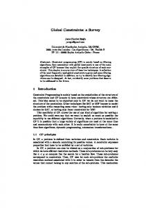
Intuitively, higher value of avgP also implies that there are fewer chances that the solver can reach deeper levels of the search tree. This value seems also to be related to unsatisfiability. To confirm this, Table 2 divides crossword instances according to both satisfiability and an avgP threshold (8%). Table 3 gives details on some representative instances. In particular, on the four crossword instances words and ogd in Table 3, the relationship between the efficiency of STR3 and the value of avgP is obvious. Finally, Figure 8 plots the relative efficiencies of STR2 against STR3 against the value of avgS (the average size of the tables during search), when considering the 658 instances of our experimental study. On the more difficult case where tables remain large (>1000 in Figure 8), STR3 can then be up to 3.6x faster and only 0.6x slower than STR2.

7

Summary and Future Work

We introduce STR3, a new GAC algorithm for table constraints that is competitive with STR2, a state-of-the art algorithm. Interestingly, STR3 is path-optimal, by being able to completely avoid unnecessary traversal of tables. We have shown that the performance of STR3 correlates to the average number of tuples remaining in the tables during search. The advantage of STR2 appears to depend largely on excessively high rates of table reduction (that is, very low avgP). As soon as the reduction rate drops below 90%, STR2 becomes much less effective. STR2 dominates on benchmarks tailor-made to suit table reduction algorithms — we have seen a surprising number of problems with tables that are virtually wiped out — but apart from these cases STR3 has the upper hand. The results in this paper exhibit a clear and actionable boundary for which exploitation of both STR2 and STR3 is obvious: a problem instance from a class with low avgP should be solved with STR2; the others should be solved with STR3. To cope with problems of unknown quality, many possibilities exist. For example, one can imagine a simple hybrid algorithm that probes the problem first by tentatively solving it for a while with STR2 while collecting data on table ratios. If it turns out that avgP exceeds a certain threshold, the algorithm may restart and switch to STR3.

Table 3: Detailed results on selected instances.

REFERENCES 100000

10000

avgS

1000

100

10

1 0

0.5

1

1.5 2 2.5 STR2 / STR3

3

3.5

4

Figure 8: The ratio cpu STR2 to cpu STR3 is plotted against avgS

(average size of tables during search). Dots correspond to instances.

[1] C. Bessiere, ‘Arc consistency and arc consistency again’, Artificial Intelligence, 65, 179–190, (1994). [2] C. Bessiere, E.C. Freuder, and J. R´egin, ‘Using constraint metaknowledge to reduce arc consistency computation’, AIJ,107,125–148,(1999). [3] C. Bessiere and J. R´egin, ‘Arc consistency for general constraint networks: preliminary results’, in Proc. of IJCAI’97, pp. 398–404, (1997). [4] C. Bessi`ere, J.-C. R´egin, R, H. C. Yap, and Y. Zhang, ‘An Optimal Coarse-Grained Arc Consistency Algorithm’, AIJ, 165(2), (2005). [5] P. Briggs and L. Torczon, ‘An efficient representation for sparse sets’, ACM Letters on Prog. Languages and Systems, 2(1–4), 59–69, (1993). [6] K. Cheng and R. Yap, ‘An MDD-based generalized arc consistency algorithm for positive and negative table constraints and some global constraints’, Constraints, 15(2), 265–304, (2010). [7] I. Gent, C. Jefferson, I. Miguel, and P. Nightingale, ‘Data structures for generalised arc consistency for extensional constraints’, in AAAI-07. [8] C. Lecoutre, ‘STR2: Optimized simple tabular reduction for table constraints’, Constraints, 16(4), 341–371, (2011). [9] C. Lecoutre and R. Szymanek, ‘Generalized arc consistency for positive table constraints’, in Proc. of CP-06, pp. 284–298, France, (2006). [10] O. Lhomme and J.C. R´egin, ‘A fast arc consistency algorithm for n-ary constraints’, in Proc. of AAAI’05, pp. 405–410, (2005). [11] R. Mohr and G. Masini, ‘Good old discrete relaxation’, in Proceedings of ECAI’88, pp. 651–656, (1988). [12] M. Moskewisz, C. Madigan, Y. Zhao, L. Zhang, and S. Malik, ‘Chaff: Engineering an efficient SAT solver’, in Proc. of DAC’01. [13] J. Ullmann, ‘Partition search for non-binary constraint satisfaction’, Information Sciences, 177, 3639–3678, (2007).