Instance Based Table Integration Algorithm for Multilingual Tables on the Web Daisuke Ikeda∗
Abstract We present an instance based table integration algorithm. A table is a set of instances of a record which consists of fields. A field is a pair of an attribute name and a sequence of attribute values of the same type. Given tables, the algorithm calculates two numerical features for each field using character codes and then finds correspondence between fields among tables. The novelty of the algorithm is that it uses the character code chart for the language in which the contents of the tables are written. This enables that a field can be represented by only two types of features. The algorithm requires neither an attribute value contained in all input tables nor attribute names. So, the algorithm is suitable for tables obtained from Web data, as long as they are written in the same language. Applying the algorithm for real Web data written in many languages, we demonstrate that the algorithm yields the accurate results and is robust for errors. The languages are Chinese, English, Germany, Japanese, and Korean.
1 Introduction An important feature of the Web is its diversity. There are a lot of types, purposes, and qualities of Web pages and they are written in many different kinds of languages. The diversity causes difficulties when we try to find, compare, and utilize wide variety of informations on the Web. In the chaotic World Wide Web, however, many sites provide a series of informations of the same type. For example, search facilities, which are provided at many Web sites, return a list search results. An online news outlet publishes article pages on the Web with the same style and structure. Many efforts have been paid to extract contents from such sites semi- or full-automatically [1, 7, 9, 18, 19]. A wrapper is a procedure which extracts the contents and generates tables from Web pages. We call such a table a wrapper table. Once a wrapper table is created, the next problem is to aggregate wrapper tables even though they are created from different sources. We can use integrated tables as a single database. Imagine that we have an integrated table of cars of various makers and that you want to buy a sedan. All you need is just to search the table. ∗ Computing and Communications Center, Kyushu University
[email protected]
In this paper, we present an algorithm to integrate wrapper tables gathered from the Web. The algorithm is very simple and utilizes only basic techniques, but ample enough to integrate diverse tables on the Web written in many languages.
1.1
Related Works
A table can be seen as a simple database. The database integration problem has been paid many attention in the field of database over the years. However, there are several essential difference between databases and wrapper tables. A database is well-structured and a schema is explicitly given. Therefore, most of integration algorithms are based on or require schema [3, 4, 14, 15]. On the other hand, a wrapper table does not have explicit schema. The original sources of the tables are markuped in HTML and do not have schema or attribute names. Therefore, methods developed in the database field are not applicable to this situation. Many query based integration systems have been proposed [3, 5, 6, 11, 15, 16] as well. Such a system receives a query, decomposes it into sub-queries for individual database, and joins results. Therefore, a schema of each database must be given to the system. In [6], the target of integration are usual Web sites instead of relational database, but the schema of a site must be described by a user. The main problem to integrate results is to determine whether two instances from different database are the same entity or not. Similarity measures are proposed [3, 16] based on the edit distance, vector space model, etc. The recent upsurge of semi-structured data poses the necessity of database integration in the new context [2, 6, 17, 20]. It is the integration of databases on the Web. The purpose seems to be similar to this paper, but the target and setting of their integration is completely different. In [2, 17], the main target is XML collections. In the viewpoint of a user, he/she can view HTML files whose original structured are destroyed even if their original sources are well-structure XML files (or relational database). In [20], the target is a usual HTML file but the proposed algorithm requires for input files to contain attribute names and for the contents to be formatted in table tags. However, there are many pages which looks like a list or table without table tags and does not have attributes names. If pages have attribute names, notations might be different from other sources.
1.2 Instance Based Algorithm We need an instance based integration algorithm because wrapper tables do not have any schema and attribute names. However, very few effort have been paid for instance based integration algorithms in the field of database. The algorithm in [4] uses attribute values to train a learning algorithm which learns the correspondence of schemata. SEMINT [12] uses partly numerical features of attribute values. Numerical features are calculated by the number of upper/lower case letters, digit, punctuation, and so on. The algorithm concludes that two fields contains the same type of data if their attribute values look like similar. Ideally, for an instance based algorithm, it would be the best way to find semantics of each field first and then to match fields using semantics instead of numerical features. For example, an algorithm judges the field containing “Daisuke Ikeda” to be the field for the persons names and the field containing “
[email protected]” to be one of their mail addresses. It seems, however, to be difficult especially in multilingual situations. Therefore, like SEMINT, it is reasonable for instance based algorithms to treat attribute values as just strings even if some of them are digit, and utilize numerical features of strings. One superiority of such numerical features is the independence from the domain of target databases. In the fields of clustering and machine learning, there are many algorithms based on numerical features [8, 10, 13]. Numerical features are used to learn classes of fields [10] and cluster documents [13]. In [10], Lerman and Minton introduced the syntactic token hierarchy, whose root has three children “PUNCT,” “ALPHANUM,” and “HTML.” And, for example “ALPHANUM” have two children, “ALPHA” which is the class for usual letter and “NUMBER” which is the class of digits. Kushmerick [8] formulate the wrapper verification problem which is, given two wrapper tables, to decide whether they contains data of the same type. If not, the algorithm concludes that the source site changed the format. To solve the problem, Kushmerick adopted nine features, such as digit/letter density, upper/lowercase density, punctuation density, length, and so on. As an an application of the algorithm, the wrapper maintenance problem is discussed in [8]. A Web site often changes its page style, so we need to find correspondence of fields between before and after the change. Ma et al. [13] also calculate a vector for each input document using the features, such as isUpperCaseLine (all alphabetics are upper case), isFirstUpperCaseLine (each word starts with upper case), startsWithDigit, and so on. They cluster documents with vector representation in a domain independent manner. These algorithms using numerical features are in fact domain independent but obviously heavily depend on languages. In described algorithms, only two types of letters, upper and lower case letters, are considered. However, in Japanese for example, we have two types of letters, Hiragana and Katakana, and one type
of Chinese characters instead of upper and lower cases.
1.3
Our Contribution
In this paper, we define the table integration problem. The problem is, given tables, to find a mapping of fields among them. Then, we present an instance based table integration algorithm to solve the problem. We represent a field of a table as a vector in two dimensional space, which we call the feature space. The novelty of the representation is its low dimensionality. This gives a unified view of heterogeneous tables. SEMINT [12] used a feature space to represent a field by a vector in 20 statistical characteristics of a database. Only 5 of them are instance based. They are minimum, maximum, average, coefficient of variance, standard deviation for non-blanks for sizes1 of all attribute values in a field. Using these characteristics, a field is converted to a vector in 20 dimensional space. Then, the algorithm clusters vectors in the space with respect to their Euclidean distance. Like SEMINT, the proposed algorithm also calculates a feature vector of a field. But, in calculation, we make use of the character code chart2 of the language used in input tables instead of sizes of attribute values. Any attribute value is treated as a string even if it is a digit and represented by the sum of all code numbers of it. “daisuke” is, for example in the ASCII (American Standard Code for Information Interchange) code, represented by 64, 61, 69, 73, 75, 6B, and 65 in hexadecimal. This representation is very natural. In fact, the programming language C does not distinguish a char (character) and an int (integer). Therefore, any languages are acceptable for input tables if the wrapper tables are written in the same language (character code chart) at a time. A character code chart is a gold mine of information. The characters of the same type occupy a successive area. The areas for different types are completely distinct. In the ASCII code, the digits occupy the area from 31 to 39, upper case letters from 41 to 5A, and lower case letters from 61 to 7A. Hiragana letters occupy from 3040 to 309F in Unicode3 and Katakana from 30A0 to 30FF. Therefore, character codes are expressive for characteristics of fields. Thus, our representation of field even in a low dimensionality works well to integrate wrapper tables. We evaluate the effectiveness and limit of the presented algorithm by experiments on 10 tables. 9 of them are wrapper tables created from real data on the Web. The other table is created from an XML collection. They are written in 5 languages, Chinese, English, Germany, Japanese, and Korean. For most datasets, the presented algorithm achieves 100% accuracy if enough instances are given. In our 1A
size is in byte. precisely, a character code chart is a character encoding scheme. 3 http://www.unicode.org/ 2 More
experiments, less than 50 instances are enough. Experiments show that the accuracy value is not affected by the contents language. Some experiments show that a limit of the algorithm. That is, the algorithm fails to match fields whose attribute values are semantically different but look similar. For example, in the list of tennis players, we have two such fields “Name” which is the field for tennis player names and “Coach” which contains also person’s (coach for a player) names. This paper is organized as follows: First of all, we define notations and the key representation of fields in Section 2. Then, we present the main algorithm in Section 3. In Section 4, we show experiments using wrapper table created from practical data written in Chinese, English, German, Japanese, and Korean.
2 Table Integration Problem A table consists of instances of a record. A record instance contains different types of data, each of which is called a field. A field is a pair of an attribute name and a sequence4 of attribute values of the same type. For a field f , we denote the number of all attribute values in f by | f |. For a table and any two fields f1 and f2 , | f1 | = | f2 |. Table 1 is a sample of table. Each column contains
Name D. Ikeda S. Hirokawa Y. Yamada ...
Table 1: Phone 2298 2301 2296 ...
Sample Table Email
[email protected] [email protected] [email protected] ...
data of the same type, and a column corresponds to a field. In this table, each field has an attribute name such as “Name,” “Phone,” and “Email.” Our algorithm does not require attribute names. Attribute names in Table 1 are only for expository purpose. In out algorithm, an attribute value is treated as a string even if it consists of only digits. For an attribute value e, |e| denotes the length of e5 and [e]i the i character of e, where 1 ≤ i ≤ |e|. Without loss of generality, we can assume that the number of input tables are restricted to be two. If three or more tables are given, first we apply an integration algorithm to any two of them, then the iteratively application to an integrated table and another input table leads to the integration of all input tables. For a table T , F(T ) denotes the set of all fields in T . We do not require any restriction on F(T 1 ) and F(T 2 ). We do no assume that tables such that F(T 1 ) ⊂ F(T 2 ) or that F(T 1 ) and F(T 2 ) are comparable might be input tables. 4 That
is, multiple values with the same value are allowed. notation is the same as the number of all attribute values of a field f . However, the difference is clear from the context. 5 This
We assume that for any field in T 1 , there exists at most one correspondent field in T 2 . Now, we define the table integration problem formally as follows: Definition 1 (Table Integration) The table integration problem is, given two tables T 1 and T 2 , to find the correspondence ( f1 , f2 ) between f1 ∈ F(T 1 ) and f2 ∈ F(T 2 ), where f1 and f2 are fields containing data of the same type.
3
Algorithm
Our algorithm receives two tables T 1 , T 2 and a character code chart C(·) as an input, where C(·) is a function from characters to integers. The algorithm first transforms all fields into vectors in 2 or 3 dimensional space using the code chart C(·). The space is called the feature space. Then, it calculates distances for all pairs of fields among the tables and finds iteratively nearest pairs of fields with respect to the Euclid distance between them.
3.1
Field Representation
The algorithm utilizes a function fieldval() which returns the vector in the feature space for a given field. This funcfunction fieldval( f : filed, C: code chart): vector begin for e in all instances of f do P ve := |e| i=1 C([e]i ) end a := average value of all ve ’s s := standard deviation of all ve ’s return (a, s) end Figure 1: Pseudo code to calculate the vector of a field tion is the key representation of the proposed algorithm. fieldval() treats an attribute value e of a field as a string and calculates the sum of character codes C(·) for all characters in e. We call this sum the feature value for an attribute value. Now, we extend the domain of C from a character to a string. For a string x, C(x) is defined to P|x| i=1 [x]i . Then the feature value for an attribute value e is C(e). The vector v for a field is v = (x, y), where x and y are the average and standard deviation value of all feature values in the field. This representation exhibits characteristics of an attribute value’s appearance. For an attribute value e, ve contains informations about both lengths and character types used in e, but omits the order of characters. Therefore, the substring information is ignored. Table 2 shows vectors for sample instances in Table 1. Note that special
Table 2: Attribute values and their feature values by the ASCII code chart Name C(·) Phone C(·) Email C(·) D. Ikeda 624 2298 213
[email protected] 2399 S. Hirokawa 980 2301 198
[email protected] 2511 Y. Yamada 850 2296 211
[email protected] 2811 ... ... ... ... ... ... characters, such as a space and punctuation, are used asis. For example, “D. Ikeda” is translated as C(D) + C(.) + C( )+C(I)+· · ·+C(a) = 68+46+32+73+· · ·+97 = 6246 . Note that a feature value only depends on one attribute value, it is not necessary for an integration algorithm to see all attribute values in a field. In this sense, a vector in this 2D feature space is locally definable. All attribute values in a field of Table 1 are basically different from each other. In general, however, there are fields containing some fixed optional values. For example, a sex is either male or female and a job title is selected from some fixed number of candidates. The standard deviation for such a field is expected to be low. It seems to be difficult distinguish such a field from another field which contains wide variety of attribute values but its standard deviation happens to be low. Here, we introduce another numerical feature for experimentally purpose. Let m be the number of different attribute values in a field f . Then, the vector v for a field f is v = (x, y, z), where x and y are the same as the 2D case, and z = | f |/m. We use | f |/m instead of m as-is because the difference of m between fields are important especially when m is too small. Note that this new feature is not defined for an attribute value. So, a vector in this new feature space is not locally definable.
procedure TableIntegrate(T 1 , T 2 : tables, C: code chart) begin foreach f1 ∈ F(T 1 ) do v1 := fieldval( f1 , C) foreach f2 ∈ F(T 2 ) do v2 := fieldval( f2 , C) d := distance between v1 and v2 h(v1 , v2 ) := d end end l := sorted list of all pairs (v1 , v2 ) by d(= h(v1 , v2 )) in increasing order for (v1 , v2 ) ∈ l report ( f1 , f2 ) are correspondent delete (p01 , p02 ) ∈ l if p01 = v1 or p02 = v2 end end
3.2
4
Mapping by Distance
The main part of the proposed algorithm is to calculate distances between vectors in the feature space and map close two vectors among two input tables as correspondent fields. The pseudo code for the algorithm is illustrated in Fig. 2. For each field f1 of T 1 , the algorithm calculate the Euclidean distance between f1 and f2 for any f2 of T 2 , and then selects iteratively a pair ( f1 , f2 ) providing the smallest distance among all pairs of fields. As the similarity of vectors, the cosine value of the vectors. If the vecoters are nomalized, we can see that the cosine value are equivalent to the Euclidian distance. But, by the preliminari experiments, normalization of vectors decrease accuracy values for matching fields. Thus, we do not adopt nomalization. Let N be the maximum number of attribute values for a field, n be the maximum length of an attribute value, and m = max{|F(T 1 )|, |F(T 2 )|}. Then, fieldval() runs in O(nN) time. It takes O(m2 ) time to calculate distances for all
Figure 2: Pseudo code of the algorithm pairs and (m2 log m) time to sort all distances. Therefore, the algorithm totally runs in O(nN + m2 log m) time.
Experiment
We implement the algorithm described in the previous section in Python and apply it to tables written in various languages. Table 3 lists all datasets with brief descriptions, where the fourth and fifth columns show the number of instances and fields in dataset, respectively. For the implemented program, tables written in any language are applicable if they are encoded in UTF-87 .
4.1
Search Engines
Dataset 1 are collected from 4 major search engines, AltaVista8 , Excite9 , Lycos10 , and Yahoo!11 . A page produced by a search engine contains multiple instances. An instance consists of titles of Web pages, URLs, and short descriptions for the pages. Therefore, the result of search 7 This
is an character encoding scheme of Unicode.
8 http://www.altavista.com/ 9 http://www.excite.com/ 10 http://www.lycos.com/
6A
code number is in decimal.
11 http://www.yahoo.com/
ID 1 2 3 4 5 6 7
Table 3: Datasets used in experiments Description Language Search results from 4 major search engines. English Search results Yahoo! Korea. Korean Search results Yahoo! China. Chinese XML database of academics in Kyushu university. Japanese Yellow Pages. Japanese Yahoo! Auction Korea. Korean List of tennis players. German
result looks like a table containing 3 fields. From each of 4 search engines, we gather about 1,000 search results (about 100 pages), and totally 4721 record instances are obtained. We collected 410 category names in advance from Yahoo! and the pages linked from the top page. We use these names as query words. When we gathered search results, we randomly chose keywords from the category names. For any combination of 4 search engines, we made a series of experiments as the number of instances are increasing. We evaluate the experiments by accuracy, that is, the number of matched field to the number all fields. The total number of fields is 18 since there are 6 combinations and each dataset has 3 fields. Table 4 shows all Table 4: Accuracy for integration tables among any two search engines in Dataset 1 size accuracy size accuracy 10 16/18 60 18/18 20 14/18 70 18/18 30 16/18 80 18/18 40 18/18 90 16/18 50 18/18 100 18/18 accuracy values, where “size” denotes the the number of files. Basically, a file in this dataset contains 10 found pages, so 10 in the size column means that 100 instances are included for both search engines of a combination. The algorithm fails to match fields when the size is small and it almost succeed for larger sizes. However, when the size is 90, the algorithm fails to match between URL and title fields. Apparently, the difference between URLs and page titles is easy for us because most URLs of found pages begin with “http://.” The algorithm folds all character codes of a string into one value when it calculates a feature value. This means that the algorithm ignores any properties of substrings appearance and their appearance orders. Nevertheless, the algorithm works very well for many data sizes. This dataset does not show any difference between 2 and 3 dimensional feature spaces. For Dataset 1, we integrate wrapper tables created from different sites. We need to see source files and define the correct mapping in advance. However, it is impossible to
# instances 4721 671 1773 497 1000 2908 227
# fields 3 4 3 6 3 4 13
construct such correct mapping for multilingual inputs. So, in the sequel, we use two tables whose instances are randomly selected from the same table. In this case, it is easy to check the correctness. Dataset 2 and 3 are also search result pages gathered from Yahoo! Korea12 and China13 , respectively. Both datasets have the same 3 fields of Dataset 1. Dataset 2 has another field14 . Table 5 shows accuracy values as the number of instances are increasing, where “size” is the number of files. Basically, each file contains 20 instances. Each size, we Table 5: Accuracy for integration tables of Dataset 2 size accuracy size accuracy 1 11/20 6 20/20 2 14/20 7 20/20 3 18/20 8 20/20 4 20/20 9 20/20 5 20/20 10 20/20 size 1 2 3 4 5
accuracy 8/20 12/20 20/20 20/20 18/20
size 6 7 8 9 10
accuracy 20/20 20/20 20/20 20/20 20/20
do experiments iteratively 5 times15 . Now, accuracy is defined to be m/(N × 5), where m is the number of matched fields during all 5 times iterations and N is the number of fields in the dataset. The above table of Table 5 is the result when the algorithm uses 2 dimensional feature space and the bellow one for 3 dimensional case. For both feature spaces, the algorithm increases accuracy values and achieves 100%. For this dataset, the new added feature slow the converge speed. For Dataset 3, the algorithm shows 100% accuracy if the input file size is greater than 3 if in the 2D feature space (see the above table of Table 3) and 2 in the 3D feature space (see the below of Table 3 ). 12 http://kr.search.yahoo.com/ 13 http://cn.search.yahoo.com/ 14 But,
the author does not know what the field is. the sequel, we make experiments in a similar manner for other datasets. 15 In
Table 6: Accuracy for integration tables of Dataset 2 size accuracy size accuracy 1 12/15 6 15/15 2 13/15 7 15/15 3 15/15 8 15/15 4 15/15 9 15/15 5 15/15 10 15/15 size 1 2 3 4 5
accuracy 12/15 15/15 15/15 15/15 15/15
size 6 7 8 9 10
accuracy 15/15 15/15 15/15 15/15 15/15
Table 7 shows all points for fields in two tables randomly extracted from Dataset 3 when the file is 10. Table 7: Points and distances for Dataset 3 Field Point URL = (2618.95, 948.87) Summary = (582382.92, 222902.47) Title = (207781.26, 114893.04) URL = (2595.70, 1018.10) Summary = (585820.57, 266668.74) Title = (225597.73, 104127.19)
number of instances is 50. In Dataset 4, several outliers of feature values are found. They are included in the fields of email address and phone number. Although almost all attribute values in these fields are written in the ASCII code, few of them are written in double-byte characters, like “daisu ke16 .” The feature value, for example, for “daisuke” is 100 + 97 + 105 + 115 + 117 + 107 + 101 = 74217 , while one for “daisuke” is 65348 + 65345 + 65353 + 65363 + 65365 + 65355 + 65349 = 457478 in Unicode. The values for such outliers are very huge. Thus, both the average and the standard deviation heavily affected by these outliers. In the above experiments, we use data cleaned by hand. We need some algorithm that eliminates automatically such outliers. We compare accuracy values between 2 and 3 dimensional feature spaces (see Table 9). The convergence size Table 9: Experiments using 3 dimensional feature space on Dataset 4 size accuracy size accuracy 10 26/30 60 30/30 20 26/30 70 30/30 30 28/30 80 30/30 40 30/30 90 30/30 50 30/30 100 30/30 is a bit smaller than 2D case. But, on the whole, the dimensionality does not affect accuracy values.
4.2 XML Database of Academics Dataset 4 consists of 497 XML files, each of which is a record instance of an academic in Kyushu University. A record contains “ID” which is a unique number, email address, phone, URL, job title, academic degree, and so on. Basically, contents are written in Japanese. An ID number is automatically generated and a job title is selected from options, so data in these two fields are clean. On the other hand, other fields are basically filled by hand. There are some blank fields, irregular data, and multiple values. Important differences from Dataset 1 are that contents are basically written in Japanese and selective fields exist such as the job title. Table 8 shows accuracy values as Table 8: Accuracy for integration tables with the same number of fields extracted from Dataset 2 size accuracy size accuracy 10 20/30 60 30/30 20 26/30 70 30/30 30 28/30 80 30/30 40 28/30 90 30/30 50 30/30 100 30/30 the number of instances are changing, where “size” is the number of instances. As the number of instances are increasing, the accuracy are increasing and converges to the perfect when the
4.3
Yellow Pages
Dataset 5 are HTML files each of which contains 20 instances. A record instance has the company name in Japanese, its phone number, and its address in Japanese. We gather randomly 50 files from Yahoo! PHONEBOOK18 and totally this dataset has 1,000 instances. The accuracy converges to 100% after the number of instances is just 20 and after that the algorithm keeps the accuracy value as 100%.
4.4 Auction Lists Dataset 6 are HTML files gathered from the auction site of Yahoo! Korea19 . An instance consists of 4 fields20 . Table 10 shows the result for this dataset. This table shows that the accuracy values in the 3 dimensional feature space converges into 100% faster than those in 2 dimensional feature space and the 3D feature space shows high accuracy values for many sizes. 16 For
all alphabets and digits in the ASCII code, we have correspondent double-byte characters in Japanese major character code charts. 17 A code number is in decimal. 18 http://phonebook.yahoo.co.jp/ 19 http://kr.list.auctions.yahoo.com/ 20 The author does not read Korean Hangeul sentences, but maybe, they are “Title,” “Price,” “Bids,” and “Time Left” like http://list. auctions.shopping.yahoo.com/.
100
2D 3D
95 90 85
accuracy
80 75 70 65 60 55 50
0
20
40
60
80 100 120 the number of instances
140
160
180
200
Figure 3: Accuracy for integration tables extracted from Dataset 7
Table 10: Accuracy for integration tables extracted from Dataset 6 in 2D (above) and 3D (bellow) feature spaces # acc. # acc. # acc. # acc. 1 14/20 6 20/20 11 20/20 16 20/20 2 18/20 7 20/20 12 20/20 17 20/20 3 19/20 8 20/20 13 20/20 18 20/20 4 19/20 9 16/20 14 20/20 19 20/20 5 19/20 10 20/20 15 20/20 20 20/20 # 1 2 3 4 5
acc. 14/20 19/20 20/20 20/20 20/20
# 6 7 8 9 10
acc. 20/20 20/20 20/20 20/20 20/20
# 11 12 13 14 15
acc. 20/20 20/20 20/20 20/20 20/20
# 16 17 18 19 20
acc. 20/20 20/20 20/20 20/20 20/20
4.5 List of Tennis Players Dataset 7 are HTML files21 each of which contains data of a tennis player. This datasets consists of 13 fields. Figure 3 shows the result for this dataset for the 2 and 3 dimensional spaces. We can not see clear disparity between two spaces. Accuracy values are relatively low in both dimensions compared to other datasets. This is because there are fields whose attribute values look similar, such as, “the date of birth” and “professional since” both including year, and “Name” and “Coach” both of which are names for a person. Their meanings are different but they look similar. 21 http://www.tennis-center.de/atp_loader.php? content=profile
5
Conclusion
We proposed a simple representation based on a character code chart for a field of the table. This representation enables to see fields in a unified view even they are from heterogeneous sites. Once we translate fields into the proposed representation, we can use any clustering algorithms to find correspondence among fields. A field is represented as a vector in just 2 or 3 dimensional space. This few dimensionality contrasts to the representation in 20 dimensional space [12]. For some datasets, 2 dimensional space achieves good accuracy, for other datasets, 3 dimensional space is better. But, on the whole, results of both spaces are similar. In other words, newly added feature, | f |/m, does not improve accuracy. We developed an algorithm that, given tables, finds correspondence fields among them. The algorithm simply maps two vectors if they are the nearest. In spite of the simplicity, the algorithm exhibits multilingual capability, domain independence, and high accuracy for tables on the Web due to the representation based on a code chart. For most cases, less than 50 instances are enough for the algorithm to achieve 100% accuracy. Tables used in experiments have simple and flat structures. The simplicity does not decrease the difficulties to integrate tables because they do not have any schema and attribute names, and contents are written in many languages. Instead of schema and attribute names, presented algorithm utilized only attribute values. This shows that it is applicable for tables on the Web, especially those created by wrapper (semi-)automatically. Obviously, there are tables which are not available for
the presented algorithm. In fact, the algorithm failed to find the correct mapping for some tables. There are two types of such failures including potential ones: One is the case that seems to be impossible for instance based algorithms. Consider two fields, one contains phone numbers and the other do fax numbers. For us human beings, it is impossible to distinguish them without attribute names. The other one is the case that would be improved by adding other features, that is increasing the dimensionality, or using other methods. Especially, we can expect that to find common substrings in a field would drastically improve the accuracy since our representation ignores the order of characters in a string. For a string s and its shuffled strings, they are transformed into the same integer. Thus, the proposed algorithm can not distinguish these strings. However, we must be cautious to add adhoc functions to the algorithm because to find common substrings or patterns is one of the main target of the Web mining and requires high computational costs. Instead, it is an interesting and important future work to find another numerical future that preserves (partially) information of the characters’ order. In the current implementation, the algorithm always maps fields even if two tables have nothing to do with each other. Therefore, another important future work is to find a good threshold for distances to refute some correspondence of fields if they do not contain the same data.
References
Modeling Web Sources for Information Integration, Proc. of the 15th National Conference on Artificial Intelligence, pp. 211–218, 1998. [7] N. Kushmerick, D. S. Weld and R. B. Doorenbos, Wrapper Induction for Information Extraction, Intenational Joint Conference on Artificial Intelligence, pp. 729–737, 1997. [8] N. Kushmerick, Regression Testing for Wrapper Maintenance, Proc. of the 16th National Conference on Artificial Intelligence (AAAI-99), pp. 74– 79, 1999. [9] K. Lerman, C. A. Knoblock and S. Minton, Automatic Data Extraction from Lists and Tables in Web Sources, Adaptive Text Extraction and Mining workshop, 2001. [10] K. Lerman and S. Minton, Learning the Common Structure of Data, Proc. of the 17th National Conference on Artificial Intelligence (AAAI-2000), pp. 26–30, 2000. [11] A. Levy, A. Rajaraman and J. Ordille, Querying Heterogeneous Information Sources Using Source Descriptions, Proc. of the 22nd International Conference on Very Large Data Bases (VLDB), pp. 251– 262, Sep. 1996.
[1] N. Ashish and C. A. Knoblock, Wrapper Generation for Semi-structured Internet Sources, Proc. of Workshop on Management of Semistructured Data, 1997.
[12] W. -S. Li and C. W. Clifton, SEMINT: A Tool for Identifying Attribute Correspondences in Heterogeneous Databases Using Neural Networks, Data and Knowledge Engineering, 33(1), 49–84, Elsevier Science, Amsterdam, April 2000.
[2] B. Chidlovskii, Schema Extraction from XML collections, International Conference on Digital Libraries, pp. 291–292, 2002.
[13] L. Ma, J. Shepherd and A. Nguyen, Document Classification vis Structure Synopses, Proc. of the 14th Australasian Database Conference, 2003.
[3] W. W. Cohen, Integration of Heterogeneous Databases Without Common Domains Using Queries Based on Textual Similarity, Proc. of the 1998 ACM SIGMOD International Conference on Management of Data, pp. 201–212, 1998.
[14] J. Madhavan, P. Bernstein and E. Rahm, Generic Schema Matching with Cupid, Proc. of the 27th International Conference on Very Large Data Bases (VLDB), pp. 49–58, Sep. 2001.
[4] A. Doan, P. Domingos and A. Y. Halevy, Reconciling Schemas of Disparate Data Sources: A Machine Learning Approach, Proc. of the 2001 ACM SIGMOD International Conference on Management of Data, pp. 509–520, 2001. [5] M. R. Genesereth, A. M. Keller and O. Duschka, Infomaster: An Information Integration System, Proc. of the 1997 ACM SIGMOD International Conference on Management of Data, pp. 539–542, 1997. [6] C. A. Knoblock, S. Minton, J. L. Ambit, N. Ashish, P. J. Modi, I. Muslea, A. G. Philpot and S. Tejada,
[15] R. J. Miller, L. M. Haas and M. A. Hern´andez, Schema Mapping as Query Discovery, Proc. of the 26th International Conference on Very Large Data Bases (VLDB), pp. 77–88, Sep. 2000. [16] A. E. Monge and C. P. Elkan, The Field Matching Problem: Algorithms and Applications Proc. of the Second International Conference on Knowledge Discovery and Data Mining, pp. 267–270, 1996. [17] L. Popa, Y. Velegrakis, R. J. Miller, M. A. Hernandez and R. Fagin, Translating Web Data, Proc. of the 28th International Conference on Very Large Data Bases (VLDB), pp. 598–609, Aug. 2002.
[18] Y. Yamada, D. Ikeda and S. Hirokawa, SCOOP: A Record Extractor without Knowledge on Input, Proc. of the Fourth International Conference on Discovery Science, Lecture Notes in Artificial Intelligence, Vol. 2226, pp. 428–487, 2001. [19] Y. Yamada, D. Ikeda and S. Hirokawa, Automatic Wrapper Generation for Multilingual Web Resources, Proc. of the 5th International Conference on Discovery Science, Lecture Notes in Computer Science, Vol. 2534, pp. 332–339, 2002. [20] M. Yoshida, K. Torisawa and J. Tsujii, A Method to Integrate Tables of the World Wide Web, Proc. of the 1st International Workshop on Web Document Analysis (WDA 2001), pp. 31–34, 2001. [21] M. Yoshida, Extracting Attributes and Their Values from Web Pages, Proc. of the ACL-02 Student Research Workshop, pp. 72–77, 2002.