Abstract. Zonal segmentation of the prostate into the central gland and peripheral zone is a useful tool in computer-aided detection of prostate cancer, because ...
A Pattern Recognition Approach to Zonal Segmentation of the Prostate on MRI Geert Litjens, Oscar Debats, Wendy van de Ven, Nico Karssemeijer, and Henkjan Huisman Radboud University Nijmegen Medical Centre Geert Grootteplein-Zuid 10, 6525GA Nijmegen, The Netherlands
Abstract. Zonal segmentation of the prostate into the central gland and peripheral zone is a useful tool in computer-aided detection of prostate cancer, because occurrence and characteristics of cancer in both zones differ substantially. In this paper we present a pattern recognition approach to segment the prostate zones. It incorporates three types of features that can differentiate between the two zones: anatomical, intensity and texture. It is evaluated against a multi-parametric multi-atlas based method using 48 multi-parametric MRI studies. Three observers are used to assess inter-observer variability and we compare our results against the state of the art from literature. Results show a mean Dice coefficient of 0.89 ± 0.03 for the central gland and 0.75 ± 0.07 for the peripheral zone, compared to 0.87 ± 0.04 and 0.76 ± 0.06 in literature. Summarizing, a pattern recognition approach incorporating anatomy, intensity and texture has been shown to give good results in zonal segmentation of the prostate. Keywords: prostate, MRI, segmentation, voxel classification, atlas.
1
Introduction
Prostate cancer is a major health problem in the Western world, with one in six men affected during their lifetime [1]. Multi-parametric magnetic resonance imaging (MPMR) has been shown to play an important role in the diagnosis of prostate cancer [2]. A typical MR exam contains T2-weighted, dynamic-contrastenhanced and diffusion-weighted imaging. Interpretation of MPMR prostate studies is challenging, and therefore the use of computer-aided diagnosis techniques has been investigated [3]. For correct interpretation of MPMR knowledge about the zonal anatomy of the prostate is required, because the occurrence and appearance of cancer is dependant on its zonal location [4]. From a radiological point of view the prostate is usually considered to have two visible zones on MRI, the central gland (CG) and the peripheral zone (PZ) [5]. We are exploring options to integrate knowledge about the zonal anatomy into CAD systems. For this automated segmentation of the zones is the first step. The availability of zonal segmentation is also mandatory for those CAD methods in literature that focus on the PZ only, as for example in [3]. N. Ayache et al. (Eds.): MICCAI 2012, Part II, LNCS 7511, pp. 413–420, 2012. c Springer-Verlag Berlin Heidelberg 2012 �
414
G. Litjens et al.
Although much research has been done on prostate segmentation [6,7], only recently the first study on segmentation of the individual zones was published by Makni et al. [8]. In their study they investigated the use of an evidential Cmeans clustering (ECM) approach to cluster voxels into their respective zones. In addition, they extended the ECM approach to incorporate the spatial relation between voxels. Using this method they obtained good results on their data set (0.87 ± 0.04 mean Dice coefficient for the central gland compared to a simultaneous truth and performance level estimation (STAPLE) obtained ground truth [9]). To the best of the authors knowledge their paper remains the only published paper evaluating prostate zonal segmentation. The purpose of this paper was to investigate a pattern recognition algorithm to segment the prostate zones. The pattern recognition approach uses several image features with a voxel classifier to detect the zones. This is a method that has been explored in many other segmentation problems. We compare it to a multi-parametric multi-atlas approach which is used to simultaneously segment the prostate and the prostate zones. Additionally, we will compare our results to inter-observer variability and the results obtained by Makni et al.[8]
2 2.1
Methods Multi-parametric Multi-atlas Segmentation
Multi-atlas segmentation is an accurate method for prostate segmentation, as has been shown by Klein et al. [6] We have chosen a similar approach, but extended it to use multi-parametric data. We evaluated the atlas method with both majority voting and STAPLE [9] to obtain the final binary segmentation. The registration of the atlases to the new case is performed using the elastix software package [10]. For the registration we use local normalized mutual information as a similarity metric. We register both the T2-weighted image and the quantitative apparent diffusion coefficient (ADC) map simultaneously. We chose to add the ADC map to the registration because it contains additional information on the zonal distribution within the prostate. In a previous experiment we investigated the added value of the ADC in zonal segmentation and we noticed that it improved performance. The cost function we then optimize can be expressed as 1 C(Tµ ; IF , IM ) = �N
i=1 ωi
N �
i ωi C(Tµ ; IFi , IM )
(1)
i=1
were C is the cost function, Tµ is the registration transformation, IF is the fixed (the unknown case) and IM the moving image (the atlas). Furthermore, ωi is the weight for each of the multi-parametric images i were i = 1 is the T2-weighted image and and i = 2 is the ADC map. We chose ω to be 0.5 for both i. The registration consists of two distinct steps. In the first step we register using only a translation transform to align the images to the new case. The second step is an elastic registration using a b-spline transformation. After the
A Pattern Recognition Approach to Zonal Segmentation of the Prostate
415
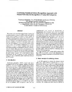
(a) T2-Weighted image
(b) Apparent diffusion coefficient map
(c) Central gland observer segmentation (Red, cyan and green for observer 1,2 and 3)
(d) Peripheral zone observer segmentation (Red, cyan and green for observer 1,2 and 3)
(e) Central gland automatic segmentation (Red, cyan and green for atlas (voting), atlas (STAPLE) and voxel classification), the STAPLE constructed ’true’ segmentation is overlayed in yellow
(f) Peripheral zone automatic segmentation (Red, cyan and green for atlas (voting), atlas (STAPLE) and voxel classification), the STAPLE constructed ’true’ segmentation is overlayed in yellow
Fig. 1. Example data set with T2-W image and ADC map in a and b and segmentation results in c, d, e and f
416
G. Litjens et al.
registration the obtained transformation is used to transform the known binary segmentations to the target image space. These can subsequently be used to construct the unknown binary segmentation. Several approaches exist in literature, of which majority voting is the simplest and best known method [6]. We compare this approach with optimizing the segmentation by using STAPLE [9]. 2.2
Voxel Classification Segmentation
For the voxel classification segmentation we determined a set of features that represent the difference between the two zones. These features can be separated into three categories: anatomy (positional), intensity and texture. For the anatomy features we use the information we know from the normal prostate composition. The peripheral zone is usually situated at the dorsal side of the prostate, getting thicker towards the apex of the prostate. We chose to model this by developing a set of three relative position and distance features. Given the whole prostate mask we can calculate a relative position in each direction for each voxel, resulting in a value between 0 and 1. We calculate this feature in the ventrodorsal direction and the craniocaudal direction. In addition, the relative distance (also between 0 and 1) to the prostate boundary is given as a feature. Two intensity features are included in the voxel classification step. The first intensity feature we use is the apparent diffusion coefficient (ADC) for each voxel, which itself should be a quantitative feature. The second intensity feature we use is a calculated T2 value for each voxel. Using the T2 relaxation time instead of the T2-weighted voxel values will make this feature much more robust to changes in scan parameters. To this end we used the following signal model equation for turbo-spin-echo sequences: � �−1 PD T2W −TE Sm Sp T2 (2) T2p = −TE log e m T2W PD Sm Sp Here T2 is the estimated T2 relaxation time, TE is the echo time for the MR pulse sequence, S the signal intensity. The superscript PD and T2W represent either the proton density weighted image or the T2-weighted image. The subscript p and m denote prostate and muscle respectively. Using this equation and a region of interest placed in a skeletal muscle we can calculate the true T2 relaxation time for each voxel given the proton density and T2-weighted images. The muscle ROI is automatically selected using a search method. Starting from the bottom slice of the T2-weighted image an Otsu threshold is performed to separate the dark areas (including the muscles) from the bright areas. We are looking for the two muscles alongside the prostate, so we suppress the center of the image with a rectangular block. Then a connected component analysis is used to find individual dark components in the image. The two largest connected components should correspond to the left and right muscle. We make sure this is the case by investigating the shape and symmetry of the two connected components. The muscle are less wide than long and they should have approximately the same shape on the left and right. We mirror the left connected component
A Pattern Recognition Approach to Zonal Segmentation of the Prostate
417
and investigate the Jaccard index with the right connected component. The minimum value for width divided by the length is 0.75 and the threshold for the Jaccard index is 0.5. The resulting connected components are eroded to ensure that the ROI is completely in the muscle. The third set of features consists of five texture features. The first two features are homogeneity and correlation calculated using the co-occurrence matrix [11]. We used 16 gray value bins for the histogram and took the average over all 2D directions. The third and fourth feature are entropy and texture strength, based on the Neighborhood Gray-Tone Difference Matrix [12]. Here also 16 gray level bins were used, in combination with an evaluation distance of 1. For all of these features the kernel size was 10x10x1 voxels. The fifth feature was the local binary pattern at each voxel [13], which was calculated over a 3x3x1 voxel neighborhood. For this feature the images were down-sampled using Gaussian re-sampling such that a 3x3x1 neighborhood corresponded to a 12x12x1 neighborhood. After calculating the features a balanced training set is constructed. Hard classification using a linear discriminant classifier is performed to obtain a binary segmentation of the central gland. To smoothen the initial boundary some post-processing is performed. Firstly, connected component analysis is used to select the largest connected component. Erosion and dilation are then performed to remove small objects attached to the segmentation. Finally the edge voxels between the central gland and the peripheral zone are selected and a thin plate spline is fitted through these voxels. This results in our final segmentation.
3
Validation
For validation we used 48 multi-parametric MR studies with manual segmentations of the whole prostate. For each case the transversal T2-weighted scan (resolution 0.6x0.6x4 mm) and the apparent diffusion coefficient map (2x2x4 mm) were used. In addition, for the voxel classification step, the proton density weighted image was used to calculate the T2 values. The ADC and proton density images were inspected to assess the alignment with the T2-weighted image. If needed, they were corrected to obtain good alignment. The ground truth was constructed by STAPLE [9] to merge the manual segmentations done by three observers. The observers made manual segmentations by indicating the zonal boundary on each T2-weighted image slice given the manual whole prostate segmentation. We validated the automatic segmentations by calculating three similarity measures: the Jaccard index (JI), the Dice similarity coefficient (DSC) and the volume difference (VD). The Jaccard index is given 1 ∩V2 | as J = |V |V1 ∪V2 | , were V1 and V2 are the automated segmentation and the STAPLE ground truth respectively. The Dice coefficient is similar to the Jaccard 2|V1 ∩V2 | . Lastly, the volume difference can index and can be expressed as D = |V 1 |+|V2 | be expressed as VD = |V1 | − |V2 |. Validation was performed in a leave-one-outmanner, thus the case to be segmented was removed from the set of atlases for the atlas method and from the training data for the voxel classification.
418
4
G. Litjens et al.
Results
In figures 2a, 2c and 2e the results of the segmentations of the central gland are presented. An example case is also shown in figure 1. We can see that the observers all perform well with respect to the STAPLE ground truth. For the segmentation methods the voxel classification approach outperforms the atlas based methods (mean DSC 0.89 ± 0.03 vs 0.80 ± 0.013 for majority voting and 0.80 ± 0.17 for STAPLE), although it is not as good as the human observers (mean DSC’s 0.95 ± 0.06, 0.97 ± 0.05, 0.96 ± 0.06). The JI and VD (figure 2b and figure 2c) show similar results. The VD results show that our methods in general under-segment the central gland. If we compare our results to those in Makni et al. [8] we perform slightly better using our voxel classification approach, as they report a mean DSC of 0.87 ± 0.04. For the peripheral zone we see similar results (figures 2b, 2d and 2f). Our pattern recognition approach outperforms the atlas based method and is relatively close to the observer scores. Here the pattern recognition approach has a mean DSC of 0.75 ± 0.07 compared to 0.82 ± 0.15, 0.89 ± 0.12 and 0.86 ± 0.11 for the observers. The atlas methods both perform poorly with respect to the peripheral zone with a mean DSC of 0.57 ± 0.19 and 0.48 ± 0.22. Compared to the state of the art we perform slightly worse, with a mean DSC of 0.76 ± 0.06 compared to our 0.75 ± 0.07.
5
Discussion
In this paper we investigated a pattern recognition approach to zonal segmentation of the prostate. We compared our method to an atlas based method and to the method published by Makni et al. Our results show that the voxel classification method outperforms the atlas based method. It also shows similar performance compared to the method published by Makni et al. We believe the pattern recognition approach outperforms the atlas-based method because it is less restrictive than an atlas, which is limited to the shapes available within the atlases. Additionally, pattern recognition allow for non-linear combination of all features, including texture features. This study also has limitations. A true comparison with the results from Makni et al. is difficult, mostly due to differences in the data used, for example in resolution. Additionally, for the atlas method we did not use the manual whole prostate segmentations because this method segments the whole prostate and the zones at the same time. This might cause some bias compared to the voxel classification approach were we did use the whole prostate manual segmentation. We did investigate using the manual whole prostate mask for the atlas method by only evaluating the registration metric within the mask. However, this approach gave worse results than not using the whole prostate mask at all. Both methods performed worst when the peripheral zone is very thin, then partial volume effects and unclear boundaries between the zones make it difficult to segment them. Finally, our voxel classification approach might be improved by incorporating additional texture features (e.g. Gaussian or Gabor based texture features) or by incorporating global information like prostate volume [8].
1
1
0.9
0.9
0.8
0.8
0.7
0.7
Dice coefficient
Dice coefficient
A Pattern Recognition Approach to Zonal Segmentation of the Prostate
0.6 0.5 0.4 0.3
0.6 0.5 0.4 0.3
0.2
0.2
0.1
0.1
0
0
Obs 1
Obs 2
Obs 3 Atlas (V) Atlas (S)
Voxel
Obs 1
(a) Dice Coefficient (CG)
Obs 2
Obs 3 Atlas (V) Atlas (S)
Voxel
(b) Dice Coefficient (PZ)
1
1
0.9
0.9
0.8
0.8
0.7
0.7
Jaccard index
Jaccard index
419
0.6 0.5 0.4 0.3
0.6 0.5 0.4 0.3
0.2
0.2
0.1
0.1
0
0 Obs 1
Obs 2
Obs 3 Atlas (V) Atlas (S)
Obs 1
Voxel
(c) Jaccard index (CG)
Obs 2
Obs 3 Atlas (V) Atlas (S) Voxel
(d) Jaccard index (PZ)
50
30 20
30
Volume Difference [mL]
Volume Difference [mL]
40
20 10 0 −10 −20 −30
10 0 −10 −20
−40
−30
−50 Obs 1
Obs 2
Obs 3 Atlas (V) Atlas (S)
(e) Volume difference (CG)
Voxel
Obs 1
Obs 2
Obs 3 Atlas (V) Atlas (S)
Voxel
(f) Volume difference (PZ)
Fig. 2. Results of the segmentation methods. The captions on the x-axes correspond to observers 1, 2 and 3, the atlas method using majority voting, the atlas method using STAPLE and the voxel classification approach.
420
G. Litjens et al.
Summarizing, a new pattern recognition approach to segment the prostate zones was presented, incorporating anatomical, intensity and texture features. It outperforms an atlas based method, is relatively close to the inter-observer performance and shows similar performance compared to the state of the art.
References 1. Siegel, R., Naishadham, D., Jemal, A.: Cancer statistics, 2012. CA Cancer J. Clin. 62, 10–29 (2012) 2. Kitajima, K., Kaji, Y., Fukabori, Y., Yoshida, K., Suganuma, N., Sugimura, K.: Prostate cancer detection with 3 T MRI: comparison of diffusion-weighted imaging and dynamic contrast-enhanced MRI in combination with T2-weighted imaging. J. Magn. Reson. Imaging 31, 625–631 (2010) 3. Chan, I., Wells, W., Mulkern, R.V., Haker, S., Zhang, J., Zou, K.H., Maier, S.E., Tempany, C.M.C.: Detection of prostate cancer by integration of line-scan diffusion, T2-mapping and T2-weighted magnetic resonance imaging; a multichannel statistical classifier. Med. Phys. 30, 2390–2398 (2003) 4. Viswanath, S.E., Bloch, N.B., Chappelow, J.C., Toth, R., Rofsky, N.M., Genega, E.M., Lenkinski, R.E., Madabhushi, A.: Central gland and peripheral zone prostate tumors have significantly different quantitative imaging signatures on 3 tesla endorectal, in vivo T2-weighted MR imagery. J. Magn. Reson. Imaging (February 2012) 5. Villeirs, G.M., Verstraete, K.L., De Neve, W.J., De Meerleer, G.O.: Magnetic resonance imaging anatomy of the prostate and periprostatic area: a guide for radiotherapists. Radiother. Oncol. 76(1), 99–106 (2005) 6. Klein, S., van der Heide, U.A., Lips, I.M., van Vulpen, M., Staring, M., Pluim, J.P.W.: Automatic segmentation of the prostate in 3D MR images by atlas matching using localized mutual information. Med. Phys. 35, 1407–1417 (2008) 7. Toth, R., Tiwari, P., Rosen, M., Reed, G., Kurhanewicz, J., Kalyanpur, A., Pungavkar, S., Madabhushi, A.: A magnetic resonance spectroscopy driven initialization scheme for active shape model based prostate segmentation. Med. Image Anal. 15, 214–225 (2011) 8. Makni, N., Iancu, A., Colot, O., Puech, P., Mordon, S., Betrouni, N.: Zonal segmentation of prostate using multispectral magnetic resonance images. Med. Phys. 38, 6093 (2011) 9. Warfield, S.K., Zou, K.H., Wells, W.M.: Simultaneous truth and performance level estimation (STAPLE): an algorithm for the validation of image segmentation. IEEE Trans. Med. Imaging 23, 903–921 (2004) 10. Klein, S., Staring, M., Murphy, K., Viergever, M.A., Pluim, J.P.W.: elastix: a toolbox for intensity-based medical image registration. IEEE Trans. Med. Imaging 29, 196–205 (2010) 11. Amadasun, M., King, R.: Textural features corresponding to textural properties. IEEE Trans. Syst. Man. Cybern. 19, 1264–1274 (1989) 12. Li, H., Giger, M.L., Olopade, O.I., Margolis, A., Lan, L., Chinander, M.R.: Computerized texture analysis of mammographic parenchymal patterns of digitized mammograms. Acad. Radiol. 12, 863–873 (2005) 13. Ojala, T., Pietikainen, M., Maenpaa, T.: Multiresolution gray-scale and rotation invariant texture classification with local binary patterns. IEEE Trans. Pattern Anal. Mach. Intell. 24, 971–987 (2002)