A PDE-based partial discharge simulator.

A PDE-based partial discharge simulator. Andrea Villa, Luca Barbieri, Marco Gondola, Andres R. Leon-Garzon, Roberto Malgesini May 30, 2017

1

Introduction

We introduce a partial discharge simulation technique fully based on the solution of a set of partial differential equations. The partial discharge (PD) analysis and simulation is a very active field of electrical engineering with many applications especially devoted to the diagnosis of the degeneration of insulating materials. Many review papers can be found in the literature, see, just to cite a few, [1, 2, 3, 4]. The PDs phenomenon is strongly related to the existence of defects in the insulating materials. They are, usually, gas-filled cavities of different shapes. Under the influence of the electric field some tiny discharges take place. In some cases the accumulated damages of the discharges tend to propagate the defect inside the material. This phenomenon is also known as treeing [4]. The PDs are both one of the main degeneration process of insulating materials and a phenomenon by which their degeneration status can be estimated. Therefore the simulation of PDs is a particularly important topic of computational applied physics. In this field, the numerical simulation has two distinct aims: to predict the shape and the evolution of the treeing and to reconstruct the evolution of partial discharges, given the geometry of a defect. In the literature two main computational approaches can be found: the stochastic modes and the deterministic ones. Let us review first the stochastic ones. One of the numerical models proposed is the dielectric breakdown model (DBM) [5]. This is mainly a simulation tool for predicting the shape of electrical trees in insulating materials. Starting from the tree root new branches are added in a random direction proportional to the intensity of the projection, in that direction, of the electric field raised to a coefficient. The value of the coefficient needs to be calibrated and it does not have a strong physical meaning. See [6] for some indications of the values usually used. The shape of the trees obtained in [5, 6] has been analyzed using the fractal theory. The DBM method, as is outlined in [7, 8], has proved to be capable of obtaining tree structures very similar to the ones observed in real insulating materials. Another very popular model is the discharge avalanche model (DAM). It was

1

first introduced in [9]. This model treats the evolution of the treeing as an accumulation of damages to the polymer structure. A PD model was added in [10] and a direct correlation with the measured data has become possible. Also some physical characteristics have been added to this class of models. In particular in [11, 12] a simple surface-resistivity model was added. The resistivity of the internal surface of the tree structures greatly affects the PDs pattern. In [11, 12] the surface resistivity is computed as a function of the accumulated damages due to PDs. In the framework of the stochastic approach different techniques are introduced. For instance in [13] a mixed BDM-DAM approach is used and in [14] an approach similar to the ones used to simulate the cellular growth is employed. From a computational viewpoint the stochastic algorithms have not a strong relationship with the underling physics of the PD. Usually only a few physical principles are included. For instance the electrostatic equation is one of these. In [12, 15] this equation is solved using the finite element method. In [16] the electric field is computed as the super-imposition of elementary charges. In [17] also the charge conservation principle is added. The stochastic models were successful in reproducing some experimental data namely the fractal structure of the treeing, as can be observed in [5, 6], and the phase-magnitude pattern described in [13, 18, 19]. An even more accurate comparison against experimental data was possible with the introduction of the deterministic models. One good reason to use a deterministic model is that the PD phenomenon itself is a nonlinear-deterministic process as is stated in a number of works [20, 21, 22, 23, 24, 25]. In particular it has been shown that the PD is a chaotic process. This behavior has been detected in many discharge phenomena using various kinds of measurement techniques: in [26] some standard electrical devices have been used to study the treeing, in [27] the light emission is recorded, in [28] the surface discharges are addressed and, finally, in [29] the ageing of dielectric fluids is studied. The nonlinear analysis of time series has made possible to calculate the nonlinear invariants of the PD dynamics [30]. For instance in [31] the state space topology of the PDs dynamics is reconstructed, in [32, 33] a correlation between the acquired signals and the type of defect is postulated and in [26] the analysis of the ageing state of the insulating material is put forward. Some examples of the deterministic models can be found in [34, 35, 36, 37]. The deterministic models mimic the main physical features of the PD process such as the discharge inception and extinction, the attachment of the charges to the surface of the defects and their detachment. As stated in [37], the deterministic models have successfully predicted the pattern, the light emission produced by the PDs and the tree structure. Although successful in predicting many aspects of the PDs-related phenomena, the deterministic approaches found in the literature use very simplified physical models. In this work we pursue a different approach based on the solution of a set of partial differential equations (PDEs). Nowadays the solution of PDEs is the principal investigation technique of applied physics. In particular the streamer model, see [38, 39, 40], can describe small scale discharges such as the 2

PDs. It is a largely more accurate model than the ones used in the literature and has a strong physical background. In this work we have complemented the streamer model to include the effects of the deposition of charged particles on the solid walls of the defect. To the best of the authors knowledge such approach has never been analysed in detail, from a numerical point of view, in the literature. In [41] the finite element method has been employed to simulate the effects of the PDs in a spherical isolated void. However the simulation of the charge dynamics and of the chemical reactions are completely neglected. There is also a relatively large literature of the simulation of gas bubbles included in insulating liquids such as water, see [42, 43, 44]. The results obtained are based on the experience gathered in other applications, see for instance [45, 46, 47], and include complex chemical reaction kinetics and the interaction of charged particles with solid insulating walls. However the analysis of the numerical schemes was not the prime concern of the cited works and in almost all the cases only two-dimensional geometries are treated. As our final aim is to simulate treeing structures we analyse and implement a full three-dimensional algorithm. We extend the numerical techniques developed in [1, 48, 49, 50, 51, 52] to include the interactions of the interface surface between the insulating bulk and the gas voids contained within. In particular we simulate the evolution of the partial discharges in a spherical void and compare the estimated induced currents on some measurement electrodes to experimental data we have acquired. Moreover we compare the qualitative behavior of the streamers in the void varying the permittivity constant of the insulating media. There is a large body of literature on this topic [42, 43, 44] to be used for comparison purposes. Let us now briefly review the structure of this paper: in Section 2 we introduce the physical model based on a set of partial differential equations. In Section 3 we discuss the discretization of the model, we decompose it in some well defined mathematical sub-problems and we asses what kind of new numerical techniques have to be used: some techniques can be directly borrowed from [52, 49, 50], some others are very specific with respect to the problem of the PDs. In Section 4 we introduce the analysis of the techniques introduced and in Section 5 we compare the numerical results to some experimental data we have acquired and with data found in the literature. Finally in Section 6 we critically review the results we have obtained.

2

Physical model

As we have outlined we aim to simulate the partial discharges that take place in arbitrary complex voids in an insulated medium. Let Ωs be the domain representing the solid insulation (usually a polymeric material) and Ωg be the domain representing the gas void. In Figure 1 we have depicted a simple configuration that has been reproduced experimentally. Let ∂Ωs and ∂Ωg be the boundaries of Ωs and Ωg respectively, moreover let Γ = ∂Ωg ∩ ∂Ωs be the interface between the two domains. In the case depicted in Figure 1 we have also Γ = ∂Ωg . We define ∂Ω = ∂Ωs /Γ as the external part of the solid insulation domain: this

3

(a) Domain Ωs ∪ Ωg .

(b) Domain Ωg .

Figure 1: An isolated void in an insulating bulk (left). The external cylinder has a radius of 5cm and is 4mm-thick. In the center of the cylinder is placed a sphere (right) with a diameter of 1mm. ⃗ s (⃗x), with ⃗x ∈ ∂Ωs , and coincides with the boundary of Ω = Ωs ∪ Ωg ∪ Γ. Let N ⃗ g (⃗x), with ⃗x ∈ ∂Ωg , be the normal unit vectors on the boundaries. N We consider the concentrations of various chemical species cp,q (t, ⃗x), with t ∈ [0, T f ], p = 1, 2, 3, 4, q = 1, . . . , Np , ⃗x ∈ Ωg , being t the time variable and T f the final simulation time. The index p spans the chemical families: p = 1 identifies electrons, p = 2 negative ions, p = 3 positive ions and p = 4 neutral species. Except for electrons, that have only one specie, each family has Np species. The number Np may vary with respect to the chosen chemical database: for instance negative ions c2,q usually include oxygen ions O2− , O− . Positive ions c3,q include N2+ , N + and, finally, neutral species c4,q often include N2 and O2 . Moreover let ∑4 ∑Np cp,q be the total concentration of the p-th family and N = p=1 Np . cp = q=1 We describe the evolution of partial discharges with the following set of partial differential equations : ( ) ( )  ∂cp,q ⃗ · ωp µp cp,q E ⃗g − ∇ ⃗ · νp ∇c ⃗ p,q = Cp,q + S ph ,  in Ωg , + ∇ p,q  ∂t  (∑ )   4 e  ⃗ ·E ⃗g =  ∇ in Ωg ,  p=1 ωp cp , ε0  ( )    ⃗ ⃗  in Ωs , ∇ · εs Es = 0, ⃗ ⃗ E = −∇ϕ, in Ω, (1)    e ⃗ ⃗ ⃗ ⃗  on Γ,  ε0 (cΓ,h − cΓ,e ) , (g · Ng = − ) εs Es · Ns + E  ∑2 ∂c  Γ,e ⃗ ⃗ ⃗ ⃗ ⃗ ⃗  c µ E · N − ν ∇c · N , on Γ, − ∇ · c µ E =  ∂t g 1 1 g τ Γ,e Γ,e Γ p=1 p p g  ( )    ∂cΓ,h + ∇ ⃗ τ · cΓ,h µΓ,h E ⃗ Γ = c3 µ3 E ⃗g · N ⃗g, on Γ, ∂t where ωp = {−1, −1, 1, 0} is the unit-charge of each family, µp is the mobility coefficient of the p-th family and νp = {ν1 , 0, 0, 0} is its diffusion coefficient: in other words we have considered only the diffusion of the electrons and we ph have neglected the others species diffusion. Cp,q and Sp,q are the chemical and the photo-ionization source terms. The first ones depend on the chosen chemical model, see for instance [53, 54, 55]. As for the photo-ionization we 4

have used a tree-term approximation, see, for instance, [56, 57, 58, 59, 60]. The ⃗ is split into two parts: the part relative to the solid insulation electric field E ⃗ s and the part E ⃗ g relative to the gas void, i.e. E(t, ⃗ ⃗x) = E ⃗ g (t, ⃗x) with ⃗x ∈ E ⃗ ⃗ Ωg and E(t, ⃗x) = Es (t, ⃗x) with ⃗x ∈ Ωs . Moreover cΓ,e , cΓ,h are the surface concentrations of electrons and holes and µΓ,e and µΓ,h are their respective ⃗ Γ is defined implicitly by the relations mobilities. The electric field on Γ, E ⃗Γ · N ⃗g = 1 E ⃗ g |Γ · N ⃗g − 1 E ⃗ s |Γ · N ⃗ s, E 2 2

⃗ Γ · ⃗τ = E ⃗ g |Γ · ⃗τ = E ⃗ s |Γ · ⃗τ , E

(2)

⃗ g = 0. Equation 2 sets where ⃗τ is any tangential unit vector such that ⃗τ · N a value for the normal electric field on the surface. Since this is discontinuous across Γ we choose the average value between the normal field in the gas and in the solid. On the contrary the tangential electric field is continuous. Finally ⃗ τ is the tangential divergence εs is the relative permittivity of the insulation, ∇ ∑4 operator on Γ, ρ = e p=1 ωp cp is the volume charge, ρΓ = e (cΓ,h − cΓ,e ) is ∑4 the surface charge, σ = e p=1 µp cp is the electrical conductivity of the bulk, σΓ = e (cΓ,h µΓ,h + cΓ,e µΓ,e ) is the surface conductivity and e is the electron charge. We point out that, by definition, σ is not null only in Ωg and vanishes in Ωs . Problem (1) must be complemented by a proper set of boundary conditions. Let ∂ΩD and ∂ΩN be a non-overlapping partition of the boundary ∂Ω: in ∂ΩD we apply Dirichlet boundary conditions and in ∂ΩN we apply Neumann boundary conditions. To be more precise, we consider the following set of boundary conditions:  A T2 w−∆w  c1 = γ µµ13 c3 + eµg |E| on Γ,  ⃗ exp(− κT ),  1   cp,q = 0, p = 2, 3, 4, q = 1, . . . , Np , on Γ, (3) b  ⃗ ⃗ on ∂ΩN ,  Es · N = EN ,   ϕ = ϕb , on ∂ΩD , where γ is the secondary emission coefficient, T is the temperature, Ag = 1.2017e6 Am−2 K −2 is a constant, κ is the Boltzmann constant, w is the material3 ⃗ b ⃗ = e |E| specific work function, ∆w(|E|) 4πε0 is the electric field correction and EN , b ϕ are two bounded given functions. In other words in (3) we have considered the combination of Schottky and secondary electron emission. The boundary conditions in (3) provide a Dirichlet condition for the drift diffusion equation of the electrons and an inflow condition for the pure drift equations of the other charged species. When discretized with a finite volume method the second condition of (3) is imposed using a ghost cell approach, see, for instance [61].

3 3.1

Numerical method Time discretization t

t

Let t0 , . . . , ti , . . . , tn be a partition of the interval [0, T ] with T = tn where nt is the total number of time steps and let ∆ti = ti+1 − ti be the time increment. 5

Given a generic function a(t, ⃗x) we define ai (⃗x) = a(ti , ⃗x), then we introduce the time discretization. We use a fully implicit approach since this technique has proven to be asymptotic preserving in the quasi neutral limit and stable, see [48, 50]. In particular we exploit the following time stepping procedure: • predictor : we solve in (ti , ti+1 ] the problem ( )  ∗,i+1/2 ∑Np i ∗,i+1/2  cp = cip + ∆ti q=1 Cp,q Yr,s cr , p = 1, 2, 3, 4,   ( )   ∗,i+1/2  ∗,i+1 i i ∗,i+1 i ⃗ ⃗  c = cp − ∆t ∇ · ωp µp cp E +   p ( ) ⃗ · νpi ∇c ⃗ ∗,i+1 ∆ti ∇ , p = 1, 2, 3, 4, p  ( )  i  ⃗ i |) µ3 ∗,i+1 Ag T 2 w−∆w(|E  c∗,i+1 c + exp − , = γ i  1 ⃗ i| κT µ1 3 eµi1 |E    ∗,i+1 cp = 0, p = 2, 3, 4, for the unknowns c∗,i+1 , p = 1, 2, 3, 4, where p { cir,s /cir , r = 1, . . . , 4, s = 1, . . . , Nr , if cir ̸= 0, i Yr,s = δr,s otherwise ;

in Ωg ,

in Ωg , on Γ, on Γ, (4)

(5)

• chemistry : we solve in the time interval (ti , ti+1 ] the following ordinary differential equation discretized with a mixed implicit-explicit Euler scheme: ( ) ( ) I O i+1/2 ph , (6) c˜i+1/2 + ∆ti Cp,q cp,q + ∆ti Sp,q = cip,q + ∆ti Cp,q ci+1/2 r,s p,q where c˜i+1/2 r,s

{ c∗,i+1 1,1 , = i+1/2 cr,s , r = 2, 3, 4, s = 1, . . . , Nr ,

(7)

O I is a proper splitting of the chemical source term Cp,q such , Cp,q and Cp,q I O that Cp,q contains all the ionization chemical reactions and Cp,q all the other reactions. Some more details can be found in [52];

• electro-drift : finally we solve the following coupled problem in (tn , tn+1 ] : ) ( ) (  i+1/2 ⃗ i+1 ⃗ gi+1 − ∆ti ∇ ⃗ · νpi ∇c ⃗ · ωp µip ci+1  = 0, in Ωg , E − cp,q + ∆ti ∇ ci+1 p,q p,q p,q   (∑ )   4 i+1 ∇ ⃗ E ⃗ gi+1 = e  , in Ωg ,  ·( p=1 ωp cp ε)0    ∇ ⃗ ⃗ i+1 = 0,  in Ωs ,  · εs Es   i+1  ⃗ ⃗ i+1 , E = −∇ϕ in Ω, ( ) i+1 i+1 e i+1 ⃗ i+1 ⃗ ⃗ ⃗  on Γ,  εs Es · Ns + Eg · N(g = − ε0 cΓ,h)− cΓ,e ,   i+1 ∑2  i+1 i+1 i i⃗ i i+1 i ⃗ i+1 ⃗ ⃗  = ∆t · Ng  p=1 cp µp Eg cΓ,e − cΓ,e − ∆t ∇τ · cΓ,e µΓ,e EΓ   i+1  i ⃗ ⃗g, −∆t ν1 ∇c ·N on Γ,  1 ( )   ci+1 − ci + ∆ti ∇ ⃗ τ · ci+1 µΓ,h E ⃗ i+1 = ∆ti ci+1 µi E ⃗ gi+1 · N ⃗g, on Γ. 3 3 Γ,h Γ Γ,h Γ,h (8) 6

Considering the first equation of (8), summing over the index q, substituting it in the second one of (8) and eliminating ci+1 from its right hand side we obtain p ⃗ ·E ⃗ gi+1 = e ∇ ε0

(

4 ∑

) ωp ci+1/2 p

e − ∆t ε0 i

p=1

(

4 ∑

( ) i+1 ⃗ ⃗ · µip ci+1 E ∇ p g

p=1

+ ∆ti

)

e ⃗ ( i ⃗ i+1 ) ∇ ν1 ∇c1 . (9) ε0

In the same way substituting the last two equations of (8) into the fifth and i+1 eliminating both ci+1 Γ,e and cΓ,h we have ⃗ i+1 · N ⃗s + E ⃗ i+1 · N ⃗g = − εs E s g

ρiΓ ∆ti i+1 ⃗ i+1 ⃗ e ⃗ i+1 · N ⃗g − σ Eg · Ng + ∆ti ν1 ∇c 1 ε0 ε0 ε0 ∆ti ⃗ ( i+1 ⃗ i+1 ) + ∇τ · σΓ EΓ . (10) ε0

Using (9) and (10) into (8) we get ) ( ) (  i+1/2 i ⃗ i+1 i⃗ i i+1 ⃗ i+1 i⃗ i+1  ∇c = 0, ∇ · ν E − ∆t ∇ · ω µ c + ∆t c − c p,q p p,q p g p,q   p,q (( ) ) p i+1/2 ( )  i i+1   ⃗ i+1 , ⃗ · 1 + ∆t σ ⃗ gi+1 = ρ ⃗ · ν i ∇c ∇ E + ∆ti εe0 ∇ 1 1  ε0 ε0  ( )  ⃗ i+1  ⃗s  ∇ · εs E = 0,    E i+1 i+1 ⃗ ⃗ = −∇ϕ (, ) i ∆ti σ i+1 i+1 ⃗ i+1 · N ⃗ ⃗ ⃗ gi+1 · N ⃗ g = − ρΓ + ∆ti e ν i ∇c ⃗g,  ε E · N + 1 + E  s s s 1 ε ε ε0 1  0 0  ( )  ∑  2 i+1 i+1 i ⃗ i+1 ⃗ i i⃗ ⃗ i+1 = ∆ti  · Ng ci+1  Γ,e − cΓ,e − ∆t ∇τ · cΓ,e µΓ,e EΓ p=1 cp µp Eg    i+1  i ⃗ ⃗  −∆t ν1 ∇c1 · Ng , (  )   ci+1 − ci + ∆ti ∇ ⃗ · ci+1 µ E ⃗ i+1 = ∆ti ci+1 µi E ⃗ i+1 · N ⃗ , Γ,h

Γ,h

τ

Γ,h

Γ,h

3

Γ

3

g

g

in Ωg , in Ωg , in Ωs , in Ω, on Γ,

on Γ, on Γ. (11)

Some of the mathematical problems that compose the numerical splitting outlined above have already been treated in previous works. For instance in [52, 48] we have worked out the first two steps of the algorithm in an efficient manner. In particular the predictor is solved with an iterative scheme that preserves the positivity of the species. The most challenging, and problem-specific, part is system (11) which is a non-linear coupled set of PDEs. We have tackled it with (1) (1) (1) a fixed point iteration, we set cp = c∗,i+1 , cΓ,h = ciΓ,h , cΓ,e = ciΓ,e and then we p

7

⃗ (l+1) , ϕ(l+1) : solve the following problem for the couple E ( ) (( ) )  ρn+1/2 ∆ti σ (l) i e ⃗ i ⃗ (l) (l+1) ⃗ ⃗  + ∆t ∇ · ν ∇c , ∇ · 1 + E =  1 1 ε) ε0 ε0 0  (   (l+1)  ⃗ ⃗  = 0,  ∇ · εs Es (l+1) (l+1) ⃗ ⃗ E = −∇ϕ ( , )  i i (l)  (l+1) ⃗  ⃗ ⃗ (l) · N ⃗g ⃗ g(l+1) · N ⃗ g = − ρΓ + ∆ti eν i ∇c εs Es · Ns + 1 + ∆tεσ0 E  1 1 ε0 ε0  ( )  i  ∆t ⃗ (l) ⃗ (l+1)  + ε0 ∇τ · σΓ E , Γ

in Ωg , in Ωs , in Ω, on Γ. (12)

Then we update the concentrations in the bulk and the concentrations of the surface charged species : ( ) ( )  (l+1) i+1/2 i⃗ i (l+1) ⃗ (l+1) i⃗ i ⃗ (l+1)  c − c + ∆t ∇ · ω µ c E − ∆t ∇ · ν ∇c = 0, in Ωg , p p p g p p  p p  ( )  ∑  (l+1) (l+1) (l+1) (l+1) (l+1) 2 c ⃗τ c ⃗ ⃗g − ci − ∆ti ∇ µΓ,e E = ∆ti cp µip E Γ,e

Γ,e

Γ,e

Γ

p=1

 ⃗ (l+1) · N ⃗g  −∆ti ν1 ∇c 1  ( )   c(l+1) − ci + ∆ti ∇ ⃗g, ⃗ (l+1) · N ⃗ τ c(l+1) µΓ,h E ⃗ (l+1) = ∆ti c(l+1) µi E 3 g 3 Γ,h Γ Γ,h Γ,h

on Γ, on Γ. (13)

We iterate until convergence and we compute the concentrations of the single species using ) ) ( ( i⃗ i ⃗ i+1 i+1/2 i⃗ i i+1 ⃗ i+1 ∇c = 0, in Ωg , (14) E − ∆t ∇ · ν ci+1 − c + ∆t ∇ · ω µ c p p,q g p p,q p,q p p,q where the concentrations ci+1 p,q , p = 1, 2, 3, 4, q = 1, . . . , Np , are now the only unknowns. Therefore we have decomposed problem (11) into the sequential solution of an elliptic problem (12) and a set of drift and drift-diffusion equations (13). In the following section we tackle these two problems and introduce the space discretization.

3.2

Space discretization

Let Ω be decomposed into nc tetrahedral elements ek , k = 1, . . . , nc , moreover let Mk = {k1 , k2 , k3 , k4 } be the set of the indices of the four elements ekj that share a face, labelled fk,j = e¯k ∩ e¯kj , with ek . Given an element k and a neighbouring element kj we define ι(k, j) as the index such that fk,j = fkj ,ι(k,j) . As regards the elements laying on the boundary we assume, for simplicity, that the boundary face is the fourth: in other words these elements have only three neighbouring elements Mk = {k1 , k2 , k3 } and fk,4 = eb,k where eb,k is a boundary element. We also denote the faces of the grid as fl with l = 1, . . . , nf where nf is the total number of faces. We can define several subsets, for instance F ext = {fl , l = 1, . . . , nf : fl ∩ ∂Ω = fl } is the set of all boundary faces. We suppose that Γ can be represented by a set of faces of the grid. Therefore, in the same way, we can define the set F Γ = {fl , l = 1, . . . , nf : fl ∩ Γ = fl } as 8

the set of all the faces belonging to Γ. All the other faces are internal faces and we denote them with F int . For greater clarity the union F Γ ∪ F int ∪ F ext is equivalent to the set of all the faces. The external faces F ext can be further divided into faces where we apply Neumann boundary conditions F N = {fl ∈ F ext : fl ∩ ∂ΩN = fl } and the set F D = {fl ∈ F ext : fl ∩ ∂ΩD = fl } where we ⃗ k be the outward pointing normal apply Dirichlet boundary conditions. Let N ⃗ k,j as the unit vector normal vector on ∂ek and, in the same way, we define N to fk,j pointing from ek to ekj . The set of the faces F Γ defines a curved twodimensional mesh, each triangle is defined as fl with fl ∈ F Γ . Similarly we define flj as the set of the three neighbouring triangles of fl ∈ F Γ and we define dl,j as the set of the three edges of fl such that f¯l ∩ f¯lj = dl,j . Once more the index ξ(l, j) is the edge index such that dl,j = dlj ,ξ(l,j) where fl ∈ F Γ . Let us now introduce the discretization space of the various building blocks that form (12) and (13). For the sake of simplicity, we clarity here the notation and drop all the iteration indices. We start rephrasing problem (12) as: ( )  ⃗ · cΩ E ⃗ = fΩ ,  ∇ in ek , k = 1, . . . , nc ,     ⃗ ⃗  E = −∇ϕ, in ek , k = 1, . . . , nc ,    c E| ⃗ ⃗ ⃗ ⃗ · N + c E| · N = 0, on fk,j ∈ F int , Ω fk,j k,j Ω fkj ,ι(k,j) kj ,ι(k,j) ( )  ⃗ f ·N ⃗ k,j + cΩ E| ⃗ f ⃗ k ,ι(k,j) − ∇ ⃗ τ · cΓ E ⃗ = fΓ , on fk,j ∈ F Γ ,  cΩ E| ·N k,j j kj ,ι(k,j)     ⃗ f ·N ⃗ k,j = F b ,  cΩ E| on fk,j ∈ F N ,  k,j N   ϕ = ϕb , on fk,j ∈ F D , (15) where { cΩ =

1+ εs ,

∆ti ε0 σ,

in Ωg , in Ωs ,

and fΓ = −

{ fΩ =

ρi+1/2 ε0

) ( ⃗ (l) , ⃗ · ν i ∇c + ∆ti εe0 ∇ 1 1

0,

ρiΓ e ⃗ ⃗ + ∆ti ν1 ∇c 1 · Ng , ε0 ε0

⃗ we can introduce Setting F⃗ = cΩ E   ⃗ ⃗ ⃗ ⃗  a(F , ψ) + b(ψ, ϕ) + c(ψ, λ) b(F⃗ , φ)   c(F⃗ , θ)

in Ωs , (16) b FNb = cΩ EN .

the weak formulation of (15) as ( ) H ⃗·N ⃗ ∈ Z, ⃗ ϕb , ∀ψ = ∂ΩD ψ ∫ = − Ω fΩ φ, ∀φ ∈ V, H H = Γ fΓ θ + ∂ΩN FNb θ, ∀θ ∈ L,

9

in Ωg ,

(17)

(18)

where  ⃗  a(F⃗ , ψ)     b(F⃗ , ϕ)  c(F⃗ , θ)     ∑nc H

k=1 ∂ek ∩∂ΩN

∫

c−1 F⃗ Ω Ω(

⃗ · ψ, ) ⃗ · F⃗ ϕ, =− Ω ∇ ∑nc (H ⃗ kθ − F⃗ · N = k=1 ∂ek /∂Ω =

∫

1 2

H

⃗ · ∇ ∂ek ∩Γ

(

cΓ ⃗ cΩ F

) ) θ +

⃗ k θ, F⃗ · N (19) {

} ⃗ ∈Z = ψ ⃗ ∈ L2 (Ω) : ψ ⃗ ∈ W r (ek ), k = 1, . . . , nc , ϕ, φ ∈ V = and where F⃗ , ψ div { } ∏ 2 1/r,v L (Ω), λ, θ ∈ L = θ ∈ fl ∈(F Γ ∪F int ) W (fl ) where v < 2 and r > 2. For more details on the continuous spaces related to the dual mixed hybridized method refer to [62]. In our case it is sufficient to consider their discrete counterparts. In particular Zh is the lowest order local Raviart-Thomas space, Vh is the space of piece-wise constant polynomials on the elements and Lh is the space of piece-wise constant polynomials on the faces belonging to F λ ≡ F int ∪F Γ ∪F N . ⃗k,j }, k = 1, . . . , nc , j = 1, 2, 3, 4 such that The space Zh has a basis {ψ I ⃗k,j · N ⃗ k,m = δj,m , k = 1, . . . , nc . ψ (20) fk,m

The space Vh can be represented by the functions { 1 in ek , φk = 0 elsewhere , where k = 1, . . . , nc . Finally the space Lh has a basis { 1 on fl ∈ F λ , θl = 0 elsewhere. Substituting the continuous functions  ∑nc ∑4 ⃗ ⃗ ⃗  F → Fh = ∑ k=1 j=1 Fk,j ψk,j , nc ϕ → ϕh = k=1 ϕk φk ,  ∑  λ → λh = l:fl ∈F λ λl θl ,

(21)

(22)

with the discrete ones i.e. ⃗→ψ ⃗k,j , k = 1, . . . , nc , j = 1, 2, 3, 4, ψ ϕ → ϕk , k = 1, . . . , nc , θ → θl , l : fl ∈ F λ , (23)

in (18) we get the following discrete saddle-point problem      TD M B T CT F  B 0 0   Φ  =  −TF  , C 0 0 L TΓ

10

(24)

where ⃗i,j , ψ ⃗k,l ), BI(i,j),k = b(ψ ⃗i,j , φk ), CI(i,j),l = c(ψ ⃗i,j , θl ), MI(i,j),J(k,l) = a(ψ I ∫ I I ( ) ⃗i,j · N ⃗ ϕb , TF k = TD I(i,j) = ψ fΩ φk , TΓ l = fΓ θ l + FNb θl , ∂ΩD

Ω

FI(i,j) = Fi,j ,

∂ΩN

Γ

Ll = λl , (25)

Φk = ϕk ,

with J(i, j) = I(i, j) = 4(i − 1) + j. Now we pass to the discretization of the first equation of (13) and, in particular we consider the evolution of electrons: i.e. the only drift-diffusion equation. The other, pure-drift, equations can be derived as a case that is simpler than the one of the electrons. Let us consider ( ) { fΩ u ⃗ ⃗ · ν ∇u ⃗ ⃗ −∇ = ∆t , in Ωg ∆t + ∇ · (uw) (26) u = fΓ , on ∂Ωg , where u represents the concentration of a family of charged particles, w ⃗ represent ⃗ g and, finally, fΩ = ci+1/2 . In particular we suppose that fΩ the drift field ωp µip E p,q and fΓ can be represented by piece-wise constant functions on the elements and ⃗ on the boundary faces, respectively. We introduce the diffusive flux ⃗q = −ν ∇u and the following mixed weak formulation of (26): ∫ ) ( ) ∫ ( H 1 ⃗− ⃗ u=− ⃗·N ⃗ ·ψ ⃗ fΓ ,  ⃗ q · ψ ∇ ψ ∀⃗q ∈ Q, Ωg ν ( ∂Ωg ) Ωg ∫ (27) ∫ ∫ ∫ uφ f ⃗ · ⃗q φ − ⃗ · (uw) − = − φ, ∀φ ∈ V, ∇ ∇ ⃗ φ − Ωg ∆t Ωg Ωg Ωg ∆t ⃗ ∈ Q and u, φ ∈ V. We have simply chosen Q = Hdiv (Ωg ) and V = where ⃗q, ψ 2 L (Ωg ). The discrete properties of (27) largely depend upon the discretization of the drift term, therefore a proper treatment is necessary. Let Qh = RT0 i.e. the lowest order Raviart-Thomas space and Vh = P0 i.e. the space of piece-wise ⃗i }, i = 1, . . . , nf,g be a basis constant functions on the elements. Then let {ψ for Qh and {φi }, i = 1, . . . , nc,g be a basis for Vh where nf,g and nc,g are, ⃗i } satisfies respectively, the number of faces and elements in Ωg . The basis {ψ the property of having a unitary flux on a face of the mesh and of having a vanishing flux on all the other faces. On the other hand the basis φi is equal to the unity only on the i-th element and it vanishes elsewhere. Substituting the continuous functions in (27) with their discrete counterparts ∑

nf,g

⃗q → ⃗qh =

u → uh =

i=1

we can state that : ∫ 1 φ ⃗ i ·⃗ φj , Mi,j = ν Ωg

∑

nc,g

⃗i , qi ψ

u i φi ,

(28)

i=1

∫ Bi,j = − Ωg

1 1 Ci,j = ∆t ∆t

(

) ⃗ j φi , ⃗ ·ψ ∇ ϕi ϕj ,

11

F

i

(

=−

) ⃗i · N ⃗ fΓ , ψ

∂Ωg

∫ Ωg

I D

1 V 1 F i= ∆t ∆t

∫

f φi , (29) Ωg

where, by a small abuse of notation, we have indicated, for instance, the mass matrix M with the same symbol as the hybridized problem (25). We will take care to clarify to which matrix, time by time, we refer. As concerns the drift term we have ∫ ∫ I 4 ∑ ( ) ⃗ · (uw) ⃗ · (uw) ⃗k ≈ ∇ ⃗ φk = ∇ ⃗ = uw ⃗ ·N |fk,j |Ck,j Φ uk , ukj , Ck,j , Ωg

ek

∂ek

j=1

(30) where ek ∈ Ωg while Ck,j =

∫

1 |fk,j |

is the interface mean drift speed and { Φ (a, b, c)

⃗ k,j , w ⃗ ·N

(31)

fk,j

a, if c ≥ 0, b, otherwise.

Scheme (30) must be slightly modified on the boundary and we get {H ( ) ⃗ k ≈ ∑3 |fk,j |Ck,j Φ uk , uk , Ck,j , uw ⃗ ·N j j=1 ∂ek /∂Ωg H ⃗ k |fk,4 |Ck,4 Φ (uk , fΓ,k , Ck,4 ) , uw ⃗ ·N ∂ek ∩∂Ωg

(32)

(33)

where fΓ,k is the k-th degree of freedom of fΓ corresponding to the boundary face fk,4 . Finally we define the matrix { ∑ Dk,k = j:kj ∈MO |fk,j |Ck,j , k (34) Dk,kj = |fk,j |Ck,j , kj ∈ MIk , and the vector FW k = −|fk,4 |Ck,4 fΓ,k ,

(35)

for all the elements ek such that Ck,4 < 0. Here we have split the set Mk into i an inflow set MIk = {kj : j ∈ [1, 4], Cp,k,j < 0} and an outflow set MO k = {kj : i j ∈ [1, 4], Cp,k,j ≥ 0}. Summing up, the discrete scheme is equal to ][ ] [ ] T M Q FD ( CB ) = , (36) U −FV − FW B − ∆t + D { } { } where Q = q1 , . . . , qnf,g and U = u1 , . . . , unc,g are the vectors of the degrees of freedom and C, from (29) and the definition of the basis {φi }, is a diagonal matrix with components Ck,k = ek . Let us, finally, review the problem of the superficial drift of the electric charges. We solve on Γ ⃗ τ · (uΓ w) uΓ + ∆t∇ ⃗ = fΓ , (37) [

where uΓ is the concentration of the surface charges at time step i + 1 and fΓ contains the concentration at the actual time step plus the forcing terms that 12

model the charge transfer from the gas-filled void and the surface. For instance, for the electrons we have fΓ = ciΓ,e + ∆ti

2 ∑

(l+1)

⃗ (l+1) − ∆ti ν1 ∇c ⃗ c(l+1) µip E p g 1

⃗g. ·N

(38)

p=1

In many cases Γ is a closed surface and boundary conditions are not required, however the model (37) can be slightly modified to take into account also these aspects. We discretize (37) using a classical finite volume scheme: uΓ,l +

3 ∑ ∆t|dl,j | j=1

with CΓ,l,j

|fl |

1 = 2|dl,j |

( ) 1 CΓ,l,j Φ uΓ,l , uΓ,lj , CΓ,l,j = |fl |

I w ⃗ · ⃗τl,j dl,j

1 − 2|dl,j |

I fΓ ,

(39)

fl

I w ⃗ · ⃗τlj ,ι(l,j) ,

(40)

dl,j

⃗ l = 0. where ⃗τl,j is the tangential vector that is normal to dl,j and satisfies ⃗τl,j · N Using definition (40) we can prove that ( ) ( ) CΓ,l,j Φ uΓ,l , uΓ,lj , CΓ,l,j = −CΓ,lj ,ι(k,j) Φ uΓ,lj , uΓ,l , CΓ,lj ,ξ(l,j) , (41) therefore scheme (39) is conservative.

4 4.1

Analysis of the method Electrostatic problem

The existence of the solution to problem (24) is directly linked with the satisfaction of the inf-sup condition of the bilinear forms b (·, ·) and c (·, ·) for the discrete spaces Zh , Vh and Lh , see [63]. The satisfaction of this property is not obvious since we have considered the surface electrical conduction and the tangential drift of charges on the surface Γ. Below we introduce some more ˆ Γ = {ek : e¯k ∩ Γ ̸= 0} nomenclature and we tackle the inf-sup condition. Let Ω be the set of the tetrahedral elements that share a face with the interface Γ, for ˆ Γ , then the sake of simplicity we suppose that, given two elements ek , ek′ ∈ Ω e¯k ∩ e¯k′ ∈ Γ. In almost all the cases the surface Γ is smooth enough and the grid is refined enough so that this property is satisfied. In any case a more complicated analysis, similar to the one used for the extended finite elements, see [64], is still possible. Moreover we suppose that, given an element ek belonging ˆ Γ , then its first face fk,1 belongs to Γ. to Ω ˆ g = Ωg /Ω ˆ Γ, Ω ˆ s = Ωs /Ω ˆ Γ and Ω ˆ Γ,g = Ωg ∩ Ω ˆ Γ, Ω ˆ Γ,s = Ωs ∩ Ω ˆ Γ. We also define Ω Moreover we outline, since we are considering the geometry depicted in Figure

13

ˆ Γ ∩ ∂Ω. Finally, for each element ek , such that ek ∈ Ω ˆ Γ = 0, we define 1, that ∂ Ω ) ( I 1 cΓ ⃗ ⃗ ⃗ ⃗ ψk,j λl zk = ψk,j · Nk λl − ∇τ · 2 ∂ek ∪Γ cΩ ∂ek /∂Ω ) ( I I ⃗k,j · N ⃗k,j ⃗ k,j − 1 ⃗ τ · cΓ ψ = ψ ∇ 2 fl cΩ fl I 1 cΓ ⃗ =1− ψk,j · ⃗τk,j . (42) 2 ∂fl cΩ I

where the indices j and l are chosen in a such a way that fk,j = fl . For the sake of simplicity we suppose that zk ̸= 0, from a numerical point of view this quantity never vanishes however, once again, if this happens, some more complex arguments can be adopted. We can now tackle the first steps for the existence proof. Proposition 1. There exists a function F⃗Γ ∈ Qh such that, given a function gΓ ∈ Lh , we have : ∫ ⃗ · F⃗Γ = 0, ∀ek ∈ Ω ˆ Γ; 1. ek ∇ 2. 3.

4.

∫ ˆg Ω

⃗ · F⃗Γ = 0; ∇

∑n c H

( ) H cΓ ⃗ Γ ⃗ k λl − 1 ⃗ F⃗Γ · N 2 ∂ek ∪Γ ∇t cΩ FΓ λl = gΓ,l , where fl ∈ F are the degrees of freedom of the function gΓ ;

k=1 ∂ek /∂Ω

and gΓ,l ∑n c H

k=1 ∂ek /∂Ω

⃗ k λl = 0, with fl ∈ F int . F⃗Γ · N

ˆ Γ,g and we define two nonProof. We consider all the elements such that ek ∈ Ω + − − ˆ ˆ empty, non-overlapping sub-groups ΩΓ,g and ΩΓ,g having n+ c and nc elements respectively. Then we define the function FΓ as  ˆ + , Fk,1 = − 1− , if ek ∈ Ω ˆ− ,  = n1+ , if ek ∈ Ω  Γ,g Γ,g nc Fk,1 c    F = −F /3, j = 2, 3, 4, e ∈ Ω ,  k,j k,1 k Γ,g   F ˆ Γ,g = −Fk,j = Fk,1 /3, j = 2, 3, 4, ek ∈ Ω kj ,ι(k,j) (43) gΓ,k −Fk,1 zk  Fk′ ,1 = ,  zk′    ˆ Γ,s ,  = −Fk′ ,1 /3, j = 2, 3, 4, ek′ ∈ Ω Fk′ ,j   F ′ ′ ˆ k ,ι(k ,j) = −Fk′ ,j = Fk,1 /3, j = 2, 3, 4, ek′ ∈ ΩΓ,s , j

ˆ Γ,s . The where the index k ′ is such that e¯k ∩ e¯k′ ̸= 0, e¯k ∩ e¯k′ ∈ Γ and ek′ ∈ Ω first claim of Proposition 1 is verified by the second and fifth relation of (43). As regards the second claim, from (43) we know that only the neighbouring ˆ Γ,g have a non-null divergence, therefore, using the third and first elements of Ω

14

equation of (43), we get ∫ ˆg Ω

∑

⃗ F⃗Γ = ∇·

4 ∫ ∑ ekj

ˆ Γ,g j=2 k:ek ∈Ω

∑ ∑ ˆ+ k:ek ∈Ω Γ,g

( ) ⃗k ,ι(k,j) = ⃗ Fk ,ι(k,j) ψ ∇· j j 4 ∑

∑

ˆ− k:ek ∈Ω Γ,g

4 ∑

Fkj ,ι(k,j) =

ˆ Γ,g j=2 k:ek ∈Ω

Fk,1 /3 =

ˆ Γ,g j=2 k:ek ∈Ω

Fk,1 +

∑

∑

Fk,1 =

ˆ Γ,g k:ek ∈Ω

∑

Fk,1 =

ˆ+ k:ek ∈Ω Γ,g

1 − n+ c

∑ ˆ− k:ek ∈Ω Γ,g

1 = 0. (44) n− c

The left hand side of the third claim, using the fourth of (43) and definition (42) is equal to Fk,1 zk + Fk′ ,1 zk′ = Fk,1 zk +

gΓ,l − Fk,1 zk ′ zk = gΓ,k . zk′

(45)

The fourth claim is a direct consequence of the third and sixth equations of (43). Then we can prove that: Proposition 2. There exists a function F⃗h ∈ Qh such that, given a function fh ∈ Vh , we have  ∫ ⃗  b(Fh , φh ) = Ω fh φh , ∀φh ∈ Vh , (46) c(F⃗h , θh ) = 0, ∀θh ∈ Lh ,  ⃗ ⃗ N Fh · N = 0, on ∂Ω . ( ) ∑ nc H ⃗ k θh and using the results F⃗ · N Proof. Introducing c˜ F⃗h , θh = k=1 ∂ek /∂Ω h in [64] we know that there exists a F⃗0 ∈ Zh such that, given a function fh ∈ Vh , we get  ∫ ⃗  b(F0 , φh ) = Ω fh φh , ∀φh ∈ Vh , (47) c˜(F⃗0 , θh ) = 0, ∀θh ∈ Lh ,  ⃗ ⃗ N F0 · N = 0, on ∂Ω . Then we define the degrees of freedom of the function gΓ ∈ Lh as gΓ,l = −c(F⃗0 , θl ), l : fl ∈ F Γ ,

(48)

and, using Proposition 1, we can determine the function F⃗Γ ∈ Qh . From [64] we know that there exists a function F⃗s ∈ Qh such that its support is contained

15

ˆ s and in Ω

 ) ∫ (  ⃗s , φh ) = ˆ ∇ ⃗ · F⃗Γ φh , ∀φh ∈ Vh ,  b( F  Ωs ⃗s , θh ) = 0, c ˜ ( F ∀θh ∈ Lh ,   F⃗ · N ⃗ ˆ s /∂ΩD , = 0, on ∂ Ω s

(49)

( ) ˆ s ∩ Γ ̸= 0, we have c F⃗s , θh = c˜(F⃗s , θh ). Since from Proposition 1 but, since Ω ∫ ⃗ · F⃗Γ = 0 we also know that there exists a function F⃗g with we know that Ωˆ g ∇ ˆ g such that support on Ω  ∫ ⃗ ⃗ ⃗  b(Fg , φh ) = Ωˆ g ∇ · FΓ φh , ∀φh ∈ Vh , c˜(F⃗g , θh ) = 0, ∀θh ∈ Lh ,  ⃗ ⃗ ˆ g. Fg · N = 0, on ∂ Ω

(50)

ˆ g ∩Γ = 0, c˜(F⃗g , θh ) = c(F⃗g , θh ). Therefore, Also in this case we have that, since Ω setting F⃗h = F⃗0 + F⃗Γ + F⃗g + F⃗s , we get b(F⃗h , φh ) = b(F⃗0 , φh ) + b(F⃗Γ , φh ) + b(F⃗g , φh ) + b(F⃗s , φh ),

(51)

now using the first of (47), (19) and the first equations of (49) and (50) we obtain ∫ ∫ ( ∫ ( ∫ ( ) ) ) ⃗ ⃗ ⃗ ⃗ ⃗ ⃗ · F⃗Γ φh = b(Fh , φh ) = fh φh − ∇ · FΓ φh + ∇ · FΓ φh + ∇ ∫

∫ fh φh −

Ω

ˆΓ Ω

(

Ω

)

Ω

⃗ · F⃗Γ φh − ∇

∫ ˆ s ∪Ω ˆf Ω

(

ˆs Ω

)

⃗ · F⃗Γ φh + ∇

∫

( ˆs Ω

ˆg Ω

∫

)

⃗ · F⃗Γ φh + ∇

ˆg Ω

(

) ⃗ · F⃗Γ φh . ∇ (52)

(

)

∫ ⃗ · F⃗Γ φh = 0 and Then, using the first claim of Proposition 1, we have Ωˆ Γ ∇ we get the first of (46). Now let us consider the following bilinear form ( ) c F⃗0 + F⃗Γ + F⃗g + F⃗s , θh = c(F⃗0 , θh ) + c(F⃗Γ , θh ) + c(F⃗g , θh ) + c(F⃗s , θh ), (53) then using (48) we have that the first term of the right hand side is equal to −gΓ , the second term, on the contrary, using the third claim of Proposition 1 is equal to gΓ : therefore the first two terms cancel out. The other two terms, ˆ s, Ω ˆ g, using the second equations of (49) and (50), and since c(·, ·) = c˜(·, ·) on Ω vanish. Therefore we get the second of (46). Passing to the last equation of (46), using the last equations of (49), (50), and since by hypothesis F⃗Γ has no contribution on ∂ΩN , we have ⃗ = (F⃗0 + F⃗Γ + F⃗g + F⃗s ) · N ⃗ = 0, ∂ΩN . F⃗h · N

16

(54)

From this last proposition we obtain directly the satisfaction of the inf-sup condition, in fact given two arbitrary, non-null, functions λh ∈ Lh , ϕh ∈ Vh we can always find a function F⃗h ∈ Zh such that : ∫ b(F⃗h , ϕh ) + c(F⃗h , λh ) = ϕ2h > 0. (55) Ω

4.2

Drift-diffusion problem

In this section we analyse the properties of scheme (36), in particular we are interested to the existence and positivity of the solution. The first step is to characterize the properties of the sub-matrices: Proposition 3. The matrix C/∆t + D has a non-singular positive inverse. Proof. First of all we outline that it is simpler to study the properties of the transpose C/∆t + DT since the positivity of the inverse does not depend on the transposition operation. We observe that, according to the definition (34) all the diagonal entries of DT are positive while all the off-diagonal entries are negative. Moreover, since we are using a conservative method, we have ∑

nc,g

DTi,j = 0,

(56)

j=1

for all the internal elements ei of the mesh such that ∂ei ∩ ∂Ωg = 0, while for all the other elements we have ∑

nc,g

DTi,j ≥ 0.

(57)

j=1

As a consequence we get nc,g ∑ T Di,i = DTi,i ≥ − DTi,j = j=1,i̸=j

∑ DTi,j .

nc,g

(58)

j=1,i̸=j

Then, since the matrix C/∆t is a positive diagonal matrix we obtain T Di,i + Ci,i /∆t >

∑ DTi,j + Ci,j /∆t .

nc,g

(59)

j=1,i̸=j

Therefore the matrix C/∆t + D is a non-singular M-matrix and its inverse is a positive matrix. The positivity of scheme (36) depends on the positivity of the inverse of the Schur complement BM−1 BT + D + C/∆t. In general the matrix BM−1 BT , though symmetric and positive definite, is not an M-matrix. However in the literature have been reported some proper, consistent, lumping techniques [65] that can be applied to the matrix M to obtain a positive diagonal lumped matrix ˜ such that the Schur complement BM ˜ −1 BT is an M-matrix. Then we get M 17

Proposition 4. Problem (36), using the consistent matrix lumping outlined above, has a unique solution and, provided that fΩ ≥ 0, fΓ ≥ 0, then U ≥ 0. Proof. Eliminating from (36) the unknown Q we get the reduced problem ( ) ˜ −1 BT + D + C/∆t U = FV + FW + BM ˜ −1 FD . BM (60) Now, using Proposition 3, we have that the matrix on the left side of (60) ˜ −1 BT + D + C/∆t is the sum of two non-singular M-matrices therefore BM is non-singular and has a positive inverse. As a consequence there exists a ˜ solution for (U and, since ) M is a diagonal matrix, we can readily compute T D −1 ˜ B U+F . Q = −M We pass now to the positivity of the solution U: since the matrix in (60) has a positive inverse we have only to check that the right hand side is positive. From the definitions of FV and FW in (29) and (35) we get directly that FV ≥ 0 and FW ≥ 0. For the last term, using (29), we have (∫ ) (I ) ( ) ( ) −1 −1 D ⃗j φi ⃗j · N ˜ F j =M ˜ ⃗ ·ψ ⃗ fΓ . Bi,j M ∇ ψ (61) j,j

j,j

Ωg

∂Ωg

⃗j · N ⃗ ̸= 0 on ∂Ωg , The right hand side of (61) is null for all the bases such that ψ therefore we get ∫ ( I ( ) ) I ( ) ⃗ j φi = ⃗j · N ⃗j · N ⃗ ·ψ ⃗ = ⃗ , ∇ ψ ψ (62) Ωg

∂ei

∂Ωg

⃗j such that ψ ⃗j · N ⃗ ̸= 0 on ∂Ωg . Plugging (62) into (61) and since fΓ is for all ψ piece-wise constant on the boundary faces of the mesh we obtain (I ) ( ) 2 ⃗j · N ˜ −1 FD j = M ˜ −1 ⃗ Bi,j M ψ fΓ,i ≥ 0, (63) j,j j,j ∂Ωg

where fΓ,i is the value of fΓ on the boundary face fi,1 . Therefore all the forcing terms in (60) are positive and we get the thesis.

5 5.1

Numerical and experimental results Comparison with experimental data

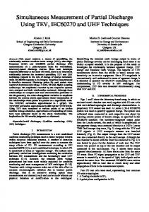
We have experimentally replicated the geometry depicted in Figure 1: two 2 mm - thick layers of polyethylene are pressed against one another with a 1 mm diameter sphere of steel between them. The pressure is applied at a temperature of nearly 80 C ◦ to diminish the residual stresses. The two layers are then separated, the steel sphere is removed and the layers are aligned precisely and glued, thus creating a cylinder with a gas-filled sphere inside it. A couple of electrodes are then placed on the cylinder as depicted in Figure 2: the upper 18

Figure 2: The experimental sensing device. electrode is energized with an AC source with a peak voltage of 4.41 kV while the other electrode, also known as the ground plate, is grounded through the R1 resistor. As partial discharges take place, some electrical charges are induced on the ground plate and an impulsive current flows through R1. This creates a potential difference across R1 which can be measured through R2 with a proper analog treatment unit whose detailed description is beyond the scope of this paper. We only point out that the analog unit behaves as a first order filter with a bandwidth of 75M Hz. The signal is then digitalized with a smart trigger device which is capable of neglecting all the un-useful data and of sampling only the evolution of the discharges. The maximum sampling period during discharge events is 1.25 ns. The experimental data can be readily compared Experimental Voltage

0

-0.2 0

1

2

3 T (µ s)

4

Computed Voltage

0.2

V (V)

V (V)

0.2

5

0

-0.2 0

6 ×104

(a)

1

2

3 T (µ s)

4

5

6 ×104

(b)

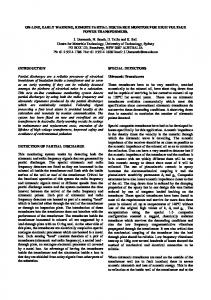
Figure 3: The measured series of current impulses (left) and the computed series (right). The signal is depicted in red while the phase of the applied voltage is depicted in black. The sine wave function is depicted only to outline the phase of discharge events. with the numerical ones since it is possible to give an estimate of the drained currents through R1. This is carried out using a duality argument [66] as has

19

been done, for instance, in [67], i.e. the induced current is computed as ∫ ⃗ ∗, Ignd = J⃗ · E

(64)

Ωg

⃗ ∗ = −∇ϕ ⃗ ∗ where J⃗ is the vector of the current density in the gas defect, E 2 ∗ is computed solving ∇ ϕ = 0 and imposing homogeneous Dirichlet boundary conditions on the top part of ∂Ω, a unitary potential on the part of the boundary corresponding to the ground plate and homogeneous Neumann conditions elsewhere. In (64) we have neglected the conduction current component since, on relatively short time scales the insulating plastic, of which Ωs is composed, behaves as a perfect insulator. The expected signal is then obtained filtering the signal Ignd /R1 with a first order filter that approximates the characteristics of the analog electronics described above. The simulation 8

×10 -11

6 4

C (C)

2 0 -2 -4 -6 -8 0

1

2

3 T (µ s)

4

5

6 ×10 4

Figure 4: The computed net charge evolution inside the sphere. The signal is depicted in red while the phase of the applied voltage is depicted in black. The sine wave function is depicted only to outline the phase of discharge events. results depend on many physical parameters. We are mainly interested in the description of the first instants after the energization of the system i.e. the period when physical parameters can be better estimated. In fact, as the discharges are accumulated, the physical properties of the solid-gas interface and of the gas that fills the void tend to vary. We have supposed that the cavity is filled with air in standard conditions. We have considered the database of [55] which takes into account molecular oxygen, nitrogen and water and nearly 50 other composed species. The initial volumetric concentrations are O2 0.2, N2 0.79, H2 O 0.01 and null for all the charged species, i.e. cΓ,h = 0, cΓ,e , cp,q = 0 with p = 1, . . . , 4, q = 1, . . . , Np . The solid material is characterized by the following physical parameters: εs = 2.25, µΓ,h = 4.0 · 10−19 m2 kV −1 µs−1 , µΓ,e = 8 · 10−20 m2 kV −1 µs−1 and γ = 0.01, w = 2.0ev. All these parameters have been extracted from [68, 67]. Though there is a large uncertainty surrounding µΓ,h , µΓ,e and w, in this case, they describe a nearly perfect insulator. We do not expect that variations of these asymptotic values (except w) will generate large variations of the solution. To cope with the uncertainty of the parameter w a sensitivity analysis has been included. To avoid any deteriora20

Experimental Voltage

0.15

0.1

V (V)

V (V)

0.1 0.05

0.05

0 -0.05 0.4

Computed Voltage

0.15

0.5

0.6

0.7 T (µ s)

0.8

0.9

0 0

1

0.1

0.2

(a)

0.3 T (µ s)

0.4

0.5

0.6

(b)

Figure 5: Comparison between a single measured (left) and computed (right) impulse. The time scales have been shifted for convenience of comparison. tion of the material we have energized the system and then readily acquired the measures within a few seconds from the power-on. A comparison between the measured and computed current impulses is included in Figure 3 showing a good agreement between them. We stress that the computed and measured impulses show an opposite polarity due to different convections of the voltage drop across R1. Both signals show, on average, a discharge for each period with a voltage amplitude between 100 and 200 mV . Also the phase of the impulse agrees quite well as this is included between the nodes of the applied voltage and the peaks. In Figure 4 the bulk charge evolution inside the gas-filled defect Computed Voltage

0

-0.1 0

1

2

3 T (µ s)

4

Computed Voltage

0.1

V (V)

V (V)

0.1

5

-0.1 0

6 ×10

0

4

(a)

1

2

3 T (µ s)

4

5

6 ×104

(b)

Figure 6: Comparison of the impulses using w = 1.6 ev (left) and w = 1.8 ev (right). The sine wave function is depicted only to outline the phase of discharge events. is depicted. This quantity is always positive since the electrons move faster than the positive ions thus creating a positive net charge that vanishes as the positive ions drift towards the walls of the defect itself. The majority of the charge impulses correspond to the current impulses of Figure 3, however it can be noticed at least a small discharge that does not have any counterpart on the chart of the induced voltage. Some tiny discharges are also observed from an experimental point of view in Figure 3. This discrepancy in the representation of small discharges could be due to the fact that our continuous representation of the concentration fields may fail just at the inception of the discharges i.e. when the concentrations are particularly low and there are a few free electrons in the cavity. In Figure 5 we have extracted two representative impulses from the

21

(a)

(b)

(c)

(d)

(e)

(f)

(g)

(h)

(i)

(j)

(k)

(l)

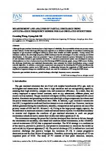
Figure 7: Time evolution of a single discharge. The first column represents a cross section of the concentration of the electrons (1020 m−3 ), the second one represents the surface charge Cm−2 and the last one represents a cross section of the electric field (kV /m). The first row corresponds to t = 31009.2867968µs, the second one to t = 31009.3600106µs, the third one to t = 31009.3715449 and the last one to t = 31024.2315265µs. experimental measures and the computed data. In particular we are comparing the impulse corresponding to the third positive peak of the applied voltage in Figure 3a with the third negative peak of the applied voltage in Figure 3b. The two impulses show very similar rise and decay times, clearly the computed signal shows a much lower noise and has a non-constant adaptive sampling time. The oscillating noise in Figure 5a makes it impossible to perform an accurate comparison of the impulse rise characteristics. However a precise comparison would require also a very detailed description of the frequency response of the signal acquisition and digitalization unit. In fact the impulse front is associated to very high frequency harmonics that are dumped by the acquisition device. As we have already pointed out, we have also performed a parametric analysis to estimate the effects of the variation of the work function w, the results are 22

shown in Figure 6. As the work function diminishes the peaks become weaker and more frequent. Even if in the first part of the third period of Figure 6a no impulse is observed at all, the associated charge plot (not depicted here) shows three distinct impulses ranging from 5 pC to 20 pC. Therefore w = 2ev seems to be one of the best candidates as, using this value, the best matching between measures and numerical predictions is observed. Much greater values of the work function are not compatible as no discharge inception is achieved. Along with the data used for validation purposes, the code produces a huge amount of data comprising the concentrations of all the charged and neutral species, the electric field and the surface charge. In Figure 7 we have depicted the evolution of the concentration of electrons, the surface charge and the electric field corresponding to the current impulse shown in Figure 5b. We have considered four steps: the first one is just before the inception and is characterized by a low concentration of the electrons. The surface charge shows a net concentration of electrons on the upper part and a concentration of holes in the lower part due to the accumulation of charges during previous discharge events. The electric field is very high since it is the superimposition of the imposed electrostatic electric field and the electric field generated by surface charges themselves. In the second time step we have depicted the formation of a streamer. The electrons, emitted by the walls, are multiplied by ionization events. They generate a large amount of positive ions, that, on the discharge time-scale, can be considered still. The ionization front becomes unstable and a streamer head is created. This is characterized by a very high concentration of electrons and a region with a high electric field just in front of it. The created new electrons drift downwards diminishing the positive surface charge on the bottom of the sphere. On the contrary, the positive ions have not enough time to interact with the upper part of the sphere. The streamer reaches the top of the sphere in the third snapshot of Figure 7 triggering an evolution of the surface charge in that region. The electric field, except a very small region near the streamer head, falls to very low values and the discharge stops. The post-discharge conditions are shown in the fourth snapshot: the electron concentration has fallen and the polarization of the sphere has been almost reversed. All the simulations have required nearly a week on a cluster parallel machine, in particular we have used a total of 24 cores: four Xeon X5675 cpus with six cores each. The complete mesh has 289995 elements 160654 of which are used to describe the spheric region Ωg where the discharges takes place.

5.2

Streamer behavior with high dielectric constant

In this test case we have used the same geometrical setup of the previous case but we have adopted a larger dielectric constant for the solid insulator. In particular we have set εs = 80. This value is similar to the relative permittivity of the water, thus this test is comparable to the research carried out considering small scale discharges in gas bubbles embedded in liquids [42, 43, 44]. Unlike those works, where two dimensional solvers have been used, we have employed a three dimensional code. As a consequence only a qualitative comparison will 23

be possible. With respect to the case discussed in Section 5.1 we have adjusted the peak voltage (3.5kV ) to remain close to the inception conditions so that the first discharge takes place nearly at the first peak of the voltage waveform. In fact since, in this case, the relative permittivity of the solid is higher, also the electric field in the void is higher. As we are mostly interested in the qualitative 4

1

V (V)

V (V)

2

0

2

0

-1 0

2000

4000

6000 8000 T (µ s)

-2 0

10000 12000

(a)

0.1

0.2

0.3 T (µ s)

0.4

0.5

0.6

(b)

Figure 8: Two discharges in a semi-period (left) and details of the second impulse (right). behaviour of the streamers we have computed only a couple of discharges as depicted in Figure 8. The discharges themselves are largely more intense since they induce a voltage that is almost ten times higher than the one described in the previous Section. The second discharge is so intense that the mean direction of the electric field in the void is reversed thus triggering an undershoot of the current impulse as shown in Figure 8b. More details can be found in Figure 9 where we have depicted the internal evolution of the electrons and the electric field in the void during the second discharge of 8. A relatively high

(a)

(b)

(c)

(d)

(e)

(f)

Figure 9: Evolution of the second discharge. In the first row the concentration of the electrons (1020 m−3 ) is depicted while in the second row the electric field (kV /m) is depicted. Each column corresponds to a time instant, the first one at t = 10341.0177984µs, the second one at t = 10341.0242156µs and the third at t = 10341.0252079µs.

24

concentration of electrons is created at the bottom of the void, the front, however, gets unstable and therefore more curved on the right side. As the front gets more curved, also the electric field increases thus leading to the formation of a streamer. Two subsequent instabilities produce two new ionization fronts: the former in the central part and the latter on the left side. The two lateral streamers remain attached to the interface between the void and the polymeric bulk. This behaviour has already been observed in [42, 43, 44] as a bigger jump of the relative dielectric constant tends to cause the streamers to attach to the boundaries. The three-dimensional simulation code we have employed makes it possible to compute the asymmetries in the propagation of the discharges too. As regards the computational cost, this simulation is largely more costly than the one discussed in Section 5.1. In fact most of the computational burden comes from the solution of the electro-drift problem which employs an iterative scheme as detailed in equation (12). Since the concentration of the charged species becomes higher, more iterations are needed to get convergence. Also the time step must be limited so that the fixed point iterations remain convergent. To be more precise, the simulation of the first two discharges depicted in Figure 8 required nearly six days which is by far a longer time tan that required for the previous test case. We also point out that a discharge event of this type would probably lead to a major distortion of the gas bubble and eventually to its break up. The maximum electric field exceeds 100M V /m which is over the maximum estimated dielectric strength of the distilled water i.e. 70M V /m [69].

6

Conclusions

In this work we have developed a numerical method for the simulation of internal partial discharges associated with isolated voids and, more generally, with internal cavities. Although the code has been validated in a two dimensional axis-symmetric geometry, it is fully three-dimensional and can handle arbitrary complex geometries. We have shown that the presented method has sound theoretical properties. These claims have been backed by the experimental results since we are capable to reproduce the main features of a train of discharges. Also the comparison of the behavior of the streamers matches the data already published in the literature. There are many physics-correlated area that must be enhanced to increase the capabilities of this numerical tool. For instance, the work function, the secondary emission coefficient and their variations with respect to the surface charge must be better understood. It would be also interesting to compare the actual results with the ones obtained with a particle method: the fluid approximation provides a suitable hypothesis during the central part of a discharge event but this could be a crude approximation just at the beginning of each discharge. In those temporal regions there are few free electrons. Even if the physical results of this method can be further improved, we still have a very good comparison between computed and experimental values especially as regards the strongest discharges. This numerical tool is currently

25

used to shed a light on the physical processes that lead to the propagation of the treeing and their diagnostics.

Acknowledgment This work has been financed by the Research Found for the Italian Electrical System under the Contract Agreement between RSE and the Ministry of Economic Development. The authors wish to thank L Barbareschi for her valuable contribution and suggestions.

References References [1] Y. Nyanteh, L. Graber, C. Edrington, S. Srivastava, D. Cartes, Overview of simulation models for partial discharge and electrical treeing to determine feasibility for estimation of remaining life of machine insulation systems, in: Electrical Insulation Conference, 2011. [2] J. C. Devins, The physics of partial discharges in solid dielectrics, IEEE Transactions on Electrical Insulation 19 (1984) 475–495. [3] L. Niemeyer, The physics of partial discharges, in: Conference on partial discharge, 1993. [4] L. A. Dissado, Understanding electrical trees in solids: from experiment to theory, in: Conference on solid dielectrics, 2001. [5] L. Niemeyer, L. Pietronero, H. J. Wiesmann, Fractal dimension of dielectric breakdown, Phys. Rev. Lett. 54 (1984) 1033–1036. [6] E. Seralathan, N. Gupta, Stochastic modeling of electric tree progression due to partial discharge activity, in: Conference on properties and applications of dielectric materials, 2006. [7] K. Wu, Z. Chengwei, G. Wu, H. Xie, A new fractal model for describing time-dependence of treeing growth, in: Symposium on Electrical Insulating Materials, 1995. [8] L. A. Dissado, Discharges and the formation of tree-shaped breakdown structures, in: Conference on Partial Discharge, 1993. [9] L. A. Dissado, P. J. J. Sweeney, Physical model for breakdown structures in solid dielectrics, Phys. Rev. B 48 (1993) 16261–16268.

26

[10] M. D. Noskov, A. S. Malinovski, M. Sack, A. J. Schwab, Self-consistent modeling of electrical tree propagation and PD activity, IEEE Transactions on Dielectrics and Electrical Insulation 7 (2000) 725–733. [11] M. D. Noskov, A. S. Malinovski, M. Sack, A. J. Schwab, Numerical investigation of insulation conductivity effect on electrical treeing, in: Conference on Electrical Insulation and Dielectric Phenomena, 1999. [12] M. Enokizono, H. Tsutsumi, Finite element analysis for discharge phenomenon, IEEE Transactions on Magnetics 30 (1994) 2936–2939. [13] A. S. Malinovski, M. D. Noskov, M. Sack, A. J. Schwab, Simulation of partial discharges and electrical tree growth in solid insulation under AC voltage, in: Conference on conduction and breakdown in solid dielectrics, 1998. [14] G. E. Vardakis, M. G. Danikas, Simulation of electrical tree propagation using cellular automata: the case of conducting particle included in a dielectric in point-plane electrode arrangement, Journal of Electrostatics 63 (2005) 129–142. [15] G. Chen, F. Baharudin, Partial discharge modelling based on a cylindrical model in solid dielectrics, in: Conference on condition monitoring and diagnosis, 2008. [16] M. D. Noskov, A. S. Malinovski, M. Sack, A. J. Schwab, The simulation of dendrite growth and partial discharges in epoxy resin, Technical Physics 72 (2002) 121–128. [17] M. D. Noskov, D. Karpov, V. Lopatin, O. Pleshkov, The simulation of the discharge channels propagation in liquinds, in: Conference on Conduction and Breakdown in Dielectric Liquids, 1996. [18] P. Morshuis, A. Cavallini, G. C. Montanari, F. Puletti, A. Contin, The behavior of physical and stochastic parameters from partial discharges in spherical voids, in: Conference on Properties and Applications of Dielectric Materials, 2000. [19] N. Hozumi, H. Nagae, Y. Muramoto, M. Nagao, H. Xie, Time-lag measurement of void discharges and numerical simulation for clarification of the factor for partial discharge pattern, in: Conference on Electrical Insulation and Dielectric Phenomena, 2000. [20] C. Yin, L. Zhou, Y. Luo, Applications of chaos theory on partial discharge detection and character analysis, in: IEEE conference on industrial technology, 2008. [21] A. A. Paithankar, A. D. Mokashi, Can PD phenomenon be analysed by deterministic chaos, in: Electrical insulation conference, 1997.

27

[22] Y. S. Lim, J. Y. Koo, Comparative analysis of partial discharge patterns from different artificial defects by means of conventional phase-resolved partial discharge analysis and a novel chaotic analysis of partial discharge, Journal of the Korean Physiscal Society 42 (2003) 755–764. [23] L. A. Dissado, Deterministic chaos in breakdown, does it occur and what can it tell us?, IEEE Transactions on Dielectrics and Electrical Insulation 9 (2002) 752–762. [24] T. Pawlowski, T. Czaszejko, Dynamics of partial discharge process from inter-spike intervals, in: IEEE Symposium on electrical insulation, 2000. [25] S. J. Dodd, J. V. Champion, Evidence for deterministic chaos in partial discharge rate measurements, in: Colloquium on PD display systems and analytical software, 1996. [26] L. Barbieri, A. Villa, R. Malgesini, A step forward in the characterization of the partial discharge phenomenon and the degradation of insulating materials through nonlinear analysis of time series, IEEE Electrical Insulation Magazine 28 (2012) 14–21. [27] H. Uehara, K. Shibuya, T. Arai, K. Kudo, Chaotic character of luminous and partial discharge phenomena during ac electrical tree propagation, in: Symposium on electrical insulating materials, 1998. [28] D. Boxue, D. Dianshuai, Z. Xiaolei, Chaos existence in surface discharge of tracking test, Trans. Tianjin. Univ. 15 (2009) 168–172. [29] Y. Mizukami, T. Inoue, T. Okamoto, K. Aihara, Nonlinear dynamical study of partial discharge phenomena, in: International conference on dielectric liquids, 1999. [30] B. Pilgram, K. Judd, A. Mees, Modeling the dynamics of nonlinear time series using canonical variate analysis, Physica D 170 (2002) 103–117. [31] T. Pawlowski, T. Czaszejko, State-space analysis of partial discharge process, in: Conference on electrical insulation and dielectric phenomena, 1999. [32] A. A. Paithankar, A. D. Mokashi, N. M. Singh, Statistical and topological characterization of PD defects, in: Electrical insulation conference, 1999. [33] M. Hoof, R. Patsch, Voltage - difference analysis, a tool for partial discharge source identification, in: IEEE Symposium on electrical insulation, 1996. [34] S. J. Dodd, N. M. Chalashkanov, J. C. Fothergill, Partial discharge patterns in conducting and non-conducting electircal trees, in: Conference on solid dielectrics, 2010. [35] T. Farr, R. Vogelsang, K. Frohlich, A new deterministic model for tree growth in polymers with barriers, in: Conference on Electrical Insulation and Dielectric Phenomena, 2001. 28

[36] K. Wu, Y. Suzuoki, T. Mizutani, H. K. Xie, The physical model for PD in tree channel and its effects on the tree growth, in: Conference on Properties and Applications of Dielectric Materials, 1997. [37] S. J. Dodd, A deterministic model for growth of non-conducting eletrical tree structures, J. Phys. D: Appl. Phys 36 (2003) 129–141. [38] L. Papageorgiou, A. C. Me, G. E. Georghiou, Three-dimensional numerical modelling of gas discharges at atmospheric pressure incorporating photoionization phenomena, J. Phys. D: Appl. Phys. 44 (2011) 045203. [39] J. Zhang, K. Adamiak, G. S. P. Castle, Numerical modeling of negativecorona discharge in oxygen under different pressures, Journal of Electrostatics 65 (2006) 174–181. [40] T. N. Tran, I. O. Golosnoy, P. L. Lewin, G. E. Ge, Numerical modelling of negative discharges in air with experimental validation, J. Phys. D: Appl. Phys. 44 (2011) 015203. [41] H. A. Illias, G. Chen, P. L. Lewin, The influence of spherical cavity surface charge distribution on the sequence of partial discharge events, J. Phys D: Appl. Phys. [42] N. Y. Babaeva, M. J. Kushner, Structure of positive streamers inside gaseous bubbles immersed in liquids, J. Phys. D: Appl. Phys. 43 (2009) 132003. [43] W. Tian, K. Tachibana, M. J. Kushner, Plasmas sustained in bubbles in water: optical emission and excitation mechanisms, J. Phys. D: Appl. Phys. 47 (2014) 055202. [44] A. Sharma, D. Levko, L. . Raja, M. S. Cha, Kinetics and dynamics of nanosecond streamer discharge in atmospheric-pressure gas bubble suspended in distilled water under saturated vapor pressure conditions, J. Phys. D: Appl. Phys. 49 (2016) 395205. [45] N. Y. Babaeva, A. N. Bhoj, M. J. Kushner, Streamer dynamics in gases containing dust particles, Plasma Sources Sci. Technol. 15 (2006) 591602. [46] Z. Xiong, M. J. Kushner, Surface corona-bar discharges for production of pre-ionizing uv light for pulsed high-pressure plasmas, J. Phys. D: Appl. Phys. 43 (2010) 505204. [47] M. J. Kushner, Modelling of microdischarge devices: plasma and gas dynamics, J. Phys. D: Appl. Phys. 38 (2005) 16331643. [48] A. Villa, L. Barbieri, M. Gondola, Towards complex physically-based lightning simulations, in: International Colloquium on Lightning and Power Systems, 2016.

29

[49] A. Villa, L. Barbieri, M. Gondola, A. R. Leon-Garzon, R. Malgesini, Stability of the discretization of the electron avalanche phenomenon, Journal of Computational Physics 296 (2015) 369–381. [50] A. Villa, L. Barbieri, M. Gondola, R. Malgesini, An asymptotic preserving scheme for streamer simulation, J. Comput. Phys. 242 (2013) 86–102. [51] A. Villa, L. Barbieri, A. Leon-Garzon, R. Malgesini, Mesh dependent stability of discretization of the streamer equations for very high electric fields, Comput. Fluids 105 (2014) 1–7. [52] A. Villa, L. Barbieri, M. Gondola, A. R. Leon-Garzon, M. Malgesini, An efficient algorithm for corona simulation with complex chemical models., J. Comput. Phys. [53] C. Chainais-Hillairet, Y. Peng, I. Violet, Numerical solutions of the EulerPoisson system for potential flows, Appl. Numer. Math. 59 (2009) 301–315. [54] A. Komuro, R. Ono, Two-dimensional simulation of fast gas heating in an atmospheric pressure streamer discharge and humidity effects, Journal of Physics D: Applied Physics 47 (15) (2014) 155202. [55] Y. Sakiyama, D. B. Graves, H.-W. Chang, T. Shimizu, G. E. Morfill, Plasma chemistry model of surface microdischarge in humid air and dynamics of reactive neutral species, J. Phys D: Appl. Phys. [56] A. Bourdon, V. P. Pasko, N. Y. Liu, S. Celestin, P. Segur, E. Marode, Efficient models for photoionization produced by non-thermal gas discharges in air based on radiative transfer and the helmholtz equation, Plasma Sources Sci. Technol. 16 (2007) 656–678. [57] E. W. Larsed, G-Thommes, A. Klar, M. Seaid, T. Gotz, Simplified Pn approzimations to the equations of radiative heat transfer and applications, Journal Of Computational Physics 183 (2002) 652–675. [58] P. Segur, A. Bourdon, E. Marode, D. Bessiers, J. H. Paillol, The use of an improved Eddington approximation to facilitate the calculation of photoionization in streamer discharges, Plasma Sources Sci. Technol. 15 (2006) 648–660. [59] J. Capeillere, P. Segur, A. Bourdon, S. Celestin, S. Pancheshnyi, The finite volume method solution of the radiative transfer equation for photon transport in non-thermal gas discharges: application to the calculation of photoionization in streamer dischages, J. Phys. D: Appl. Phys. 41 (2008) 234018. [60] S. V. Pancheshnyi, S. M. Starikovskaia, A. Y. Starikovskii, Role of photoionization processes in propagation of cathode-directed streamer, J. Phys. D: Appl. Phys. 34 (2001) 105–115.

30

[61] A. Villa, L. Barbieri, R. Malgesini, Ghost cell boundary conditions for the Euler equations and their relationships with feedback control, Communications in Applied and Industrial Mathematics 3 (1). [62] D. Arnold, F. Brezzi, Mixed and nonconforming finite element methods: Implementation, postrocessing and error estimates., Math. Modeling and Numer. Anal. 19 (1) (1985) 7–32. [63] M. Fortin, F. Brezzi, Mixed and hybrid finite element methods, Springer, 1991. [64] C. D’Angelo, A. Scotti, A mixed finite element method for darcy flow in a fractured porous media with non-matching grids, ESAIM: Mathematical Modelling and Numerical Analysis 46 (2) (2011) 465–489. [65] S. Micheletti, R. Sacco, F. Saleri, On some mixed finite element methods with numerical integration, SIAM J. Sci. Comput 23 (1) (2001) 245–270. [66] H. Zhong, Review of the shockleyramo theorem and its application in semiconductor gamma-ray detectors, Nuclear Instruments and Methods in Physics Research Section A: Accelerators, Spectrometers, Detectors and Associated Equipment. [67] T. N. Tran, I. O. Golosnoy, P. L. Lewin, G. E. Georghiou, Numerical modelling of negative discharges in air with experimental validation, J. Phys D: Appl. Phys 44 (2011) 015203. [68] Y. V. Serdyuk, S. M. Gubanski, Computer modeling of interaction of gas discharge plasma with solid dielectric barriers, IEEE Transactions on Dielectrics and Electrical Insulation. [69] W. M. Haynes, Handbook of chemistry and physics, CRC, 2016.

31