Figure 1: A metric derived from our model, that predicts the perceived difference (
right) ... Depth perception is an important skill that received much atten-.
A Perceptual Model for Disparity Tobias Ritschel2,3 Informatik
2 Télécom
Karol Myszkowski1 3 Intel
ParisTech
Hans-Peter Seidel1
Visual Computing Institute
Noi s e Qua nz e
Di s t or t e ddi s pa r i t y
S t e r e oc ont e nt
Di s pa r i t y
1 MPI
Elmar Eisemann2
Compr e s s
Piotr Didyk1
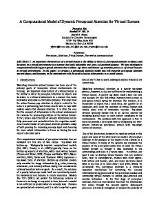
Figure 1: A metric derived from our model, that predicts the perceived difference (right) between original and distorted disparity (middle).
Abstract Binocular disparity is an important cue for the human visual system to recognize spatial layout, both in reality and simulated virtual worlds. This paper introduces a perceptual model of disparity for computer graphics that is used to define a metric to compare a stereo image to an alternative stereo image and to estimate the magnitude of the perceived disparity change. Our model can be used to assess the effect of disparity to control the level of undesirable distortions or enhancements (introduced on purpose). A number of psycho-visual experiments are conducted to quantify the mutual effect of disparity magnitude and frequency to derive the model. Besides difference prediction, other applications include compression, and re-targeting. We also present novel applications in form of hybrid stereo images and backward-compatible stereo. The latter minimizes disparity in order to convey a stereo impression if special equipment is used but produces images that appear almost ordinary to the naked eye. The validity of our model and difference metric is again confirmed in a study. CR Categories: I.3.3 [Computer Graphics]]: Picture/Image generation—display algorithms,viewing algorithms; Keywords: Perception; Stereo Links: DL PDF W EB
1
configurations which is crucial for the understanding of a scene. For this reason, conveying depth has challenged artists for many centuries [Livingstone 2002] and has been identified as an important problem in contemporary computer graphics [Wanger et al. 1992; Matusik and Pfister 2004; Lang et al. 2010]. There are many known and unknown high-level processes involved in stereo perception. In this work, we will exclusively consider binocular disparity, a low-level, pre-attentive cue, attributed to the primary visual cortical areas [Howard and Rogers 2002, Chapter 6] which is one of the most important stereo cues [Cutting and Vishton 1995]. Different from previous studies of disparity [Howard and Rogers 2002, Chapter 19], we propose a model to account for the mutual effect on perceived depth of frequency and magnitude changes in disparity, measured with a consistent set of stimuli. Applications of our model include a stereo-image-difference metric, disparity re-targeting, compression and two novel applications: backward-compatible stereo and hybrid stereo images. Backwardcompatible stereo minimizes disparity in order to show an almost ordinary appearance when observed without special equipment, but conveys a stereo impression if special equipment is used. Hybrid stereo images depict different stereo content when observed from different distances. Finally, the metric is validated in another perceptual study. We make the following contributions: • Measurement of detection and discrimination disparity thresholds, depending on magnitude and frequency of disparity;
Introduction
The human visual system (HVS) uses an interplay of many cues [Palmer 1999; Howard and Rogers 2002] to estimate spatial
• A perceptual model and a resulting metric to predict perceived disparity changes; • A study to validate the effectiveness of our findings; • Various application scenarios (including two novel ones: backward-compatible stereo and hybrid stereo images). We report a concrete model for standard stereo equipment, but we expose all details to build new instances for different equipments.
2
Background
Here, we give background information on stereoscopic vision and show analogies between apparent depth and brightness perception.
2.1
Depth Perception
Depth perception is an important skill that received much attention [Howard and Rogers 2002; Palmer 1999]. The estimation of observer-object and inter-object distances is one of the most important tasks of the HVS. Its exploration is of relevance in many computer graphics contexts, including virtual reality and movies [Wanger et al. 1992; Lang et al. 2010]. Depth Cues The HVS relies on a large variety of depth cues, which can be categorized [Palmer 1999] as pictorial information (occlusions, perspective foreshortening, relative and familiar object size, texture and shading gradients, shadows, aerial perspective), as well as, dynamic (motion parallax), ocular (accommodation and vergence), and stereoscopic information (binocular disparity). The HVS exhibits different sensitivity to these depth cues (which may strongly depend on the object’s distance to the eye [Cutting and Vishton 1995]) and integrates the occasionally contradictory information. Dominant cues may prevail or a compromise 3D scene interpretation (in terms of cues likelihood) is perceived [Palmer 1999, Chapter 5.5.10].
is one of the strongest and most compelling depth cues, where the HVS reconstructs distance by the amount of lateral displacement (binocular disparity) between the object’s retinal images in the left and right eye [Palmer 1999, Chapter 5.3]. Through vergence both eyes can be fixated at a point of interest (e. g., F in Fig. 2), which is then projected with zero disparity onto corresponding retinal positions. The disparity at P for the fixation point F is measured as the difference of vergence angles ω − θ (Fig. 2). Note that this is different from the computer vision meaning of this word, where, disparity describes the lateral distance (e. g., in pixels) of a single object inside two images (Fig. 2). We will use “disparity” in the sense of perception literature and data, while “pixel disparity” refers to the vision definition. In our work we consider only horizontal disparities as they have stronger contribution to the depth perception than other, e. g., vertical disparities [Howard and Rogers 2002, Chapter 20.3]. Stereopsis
Comfort starts
Eyes
Pixel disp.
Comfort ends ω
θ
Vergence F P Horopter
Figure 2: Binocular vision. Retinal images can be fused only in the region around the horopter, called Panum’s fusional area, and otherwise double vision (diplopia) is experienced. The fusion depends on many factors such as individual differences, stimulus properties (better fusion for small, strongly textured, well-illuminated, static patterns), and exposure duration. Binocular Fusion
Stereopsis is a low-level cue, which can be conveniently studied in isolation from other depth cues by means of random-dot stereograms as proposed by Julesz [1971]. Interestingly, disparity shares a number of properties with brightness perception [Brookes and Stevens 1989; Lunn and Morgan 1995; Bradshaw and Rogers 1999]. The disparity detection threshold depends on the spatial frequency of a corrugated in-depth pattern with a peak sensitivity around 0.3–0.5 cpd (cycles-per-degree). The disparity sensitivity function (DSF), which is analogous to the contrast sensitivity function (CSF) in the luminance domain, has the Disparity Sensitivity
familiar inverse “u”-shape with a cut-off frequency around 3 cpd [Bradshaw and Rogers 1999, Fig. 1]. Also, for larger-amplitude (suprathreshold) corrugations [Ioannou et al. 1993], the minimal disparity changes that can be discriminated (discrimination thresholds) exhibit a Weber’s Law-like behavior and increase with the amplitude of corrugations [Howard and Rogers 2002, Fig. 19.24 d]. Analogous to luminance maladaptation, where the HVS can hardly adopt to rapidly changing illumination conditions, disparity perception is subject to a similar mechanism. Disparity detection and discrimination thresholds are increasing when corrugated patterns are moved away from the zero-disparity plane [Blakemore 1970, Fig. 6]. The larger the pedestal disparity (i. e., the further the pattern is shifted away from zero-disparity) the higher are such thresholds. Techniques used in spatial contrast vision, such as masking and adaptation, provide clear evidence that the CSF shape is an envelope of responses for a number of independent channels, which are tuned to different spatial frequencies [Daly 1993]. The same conclusion can be drawn when similar techniques are employed with respect to disparity (refer to [Howard and Rogers 2002, Chapter 19.6.3d] for the survey of relevant experiments). The independent channel bandwidth for disparity modulation has not been clearly established, but existing estimates suggest the range of 1–3 octaves. Visual Channels for Disparity
Apparent depth is dominated by the distribution of disparity contrasts rather than absolute disparities [Brookes and Stevens 1989], which is similar to apparent brightness which is governed by contrasts rather than absolute luminance. While the precise relationship between apparent depth and disparity features is not fully understood, depth is perceived most effectively at surface discontinuities and curvatures, where the second order differences of disparity are non-zero. This means that binocular depth triggered by disparity gradients (as for slanted planar surfaces) is weak and, in fact, dominated by the monocular interpretation [Brookes and Stevens 1989]. As confirmed by the Craik-O’Brien-Cornsweet illusion for depth [Anstis and Howard 1978; Rogers and Graham 1983], where a strong apparent depth impression arises at sharp depth discontinuities and is maintained over regions where depth is actually decaying towards equidistant ends. Recently, it was found that effects associated with lateral inhibition of neural responses (such as Mach bands, the Hermann grid, and simultaneous contrast illusions) can be readily observed for disparity contrast [Lunn and Morgan 1995]. Disparity Contrast
2.2
3D Image Quality Metrics
While it has been recognized that image quality metrics for conventional 2D images (see [Wang et al. 2004] for a survey) should be extended to meaningfully predict the perceived quality of stereoscopic 3D images, relatively little research addresses this issue. Meesters et al. [2004] postulate a multidimensional 3D-imagequality model that incorporates perceptual factors related to disparity distortions (focus of this work), visual comfort, and 3D image impairments. In practice, all these factors are considered in isolation and existing quality metrics are mostly driven by 3D image compression applications. A comprehensible 3D-image-quality metric seems a distant goal. Visual Comfort in 3D displays strongly depends on interactions between eye vergence and accommodation which tends to maintain the display screen within the depth of focus (DOF) that roughly falls into the range of ±0.3 diopters [Hoffman et al. 2008]. Accommodation-vergence models incorporating dualparallel feedback-control systems exist (see [Lambooij et al. 2009]
for a short survey), but focus rather on dynamic interactions. Our perceived disparity model does not account for accommodation, but we focus our measurements and applications on disparity ranges that do not cause visual discomfort due to blur and diplopia. Meesters et al. [2004] provide a detailed survey of techniques dealing with 3D-image impairments induced by camera configurations, image compression, or display technology. These impairments are either aspects of higher-level (cognitive) aspects of the HVS, which are beyond the scope of this work, or affect mostly the 3D appreciation and visual discomfort and are less related to depth perception. 3D Image Impairments
of stereo content shown on stereoscopic displays is often caused by wrong viewing distance or position, which results in distorted shape perception. Recent work by Held et al. [2008] presents a mathematical model for predicting these distortions. However they do not address the problem of detecting visibility or strength of those changes which is crucial for our applications. Misperceptions
MPEG and JPEG compression artifacts in the color information, affect image quality, but have little influence on perceived depth [Seuntiens et al. 2006]. Therefore we do not consider them in this work. Sazzad et al. [2009] developed a non-reference stereoscopic image quality metric which combines the estimate of blockiness and blur with a disparity measure. Benoit et al. [2008] report significant correlation with subjective mean-opinion-score (MOS) data for stereo images, when the disparity error is incorporated into standard 2D image metrics (in particular in conjunction with the structural similarity index (SSIM) [Wang et al. 2004]). But, in all cases, pixel disparity errors are measured in absolute scale without taking perceived disparity distortion into account which is one of our main goals. Compression Artifacts
2D Image Quality Metrics focus on near-threshold detection [Daly 1993], supra-threshold discrimination [Lubin 1995], functional differences [Ramanarayanan et al. 2007], and structural differences [Wang et al. 2004]. Since we intend to measure suprathreshold depth distortions and evaluate their magnitude in perceptually meaningful scales, the VDM metric [Lubin 1995] is closest to our needs. Analogously, we consider the DSF, disparity masking, disparity channel decomposition, and pooling of perceived disparity differences over such channels to derive a per-pixel difference map. The VDM metric relies on the contrast transducer, which represents a hypothetical response of the HVS to a given contrast [Wilson 1980; Lubin 1995; Mantiuk et al. 2006]. The following section describes a perceptual experiment to derive disparity transducers for selected frequencies of corrugated spatial patterns leading to to a perceptual linearization of physical disparity.
3
Method
To derive disparity transducers, we need precise detection and discrimination thresholds that cover the full range of magnitudes and spatial frequencies of corrugated patterns that can be seen without causing diplopia. While some disparity detection data is readily available [Bradshaw and Rogers 1999; Tyler 1975] (see [Howard and Rogers 2002, Chapter 19.6.3] for a survey), we are not aware of any set of densely measured discrimination thresholds. The closest experiment to ours has been performed by Ioannou et al. [1993] where observers matched peak-to-trough corrugations of various spatial frequencies to a variable amplitude-reference corrugation of fixed intermediate frequency. Only three suprathreshold amplitudes (up to 8 arcmin) have been investigated [Howard and Rogers
2002, Fig. 19.24 d], and we are more interested in the disparitydifference discrimination within the same frequency to account for intra-channel masking. Furthermore, existing measurements are often performed with sophisticated optical setups (e. g., [Blakemore 1970]), whereas we wanted to acquire data for modern, inexpensive 3D displays, which are also used in our applications (Sec. 6). We allow for free eye motion in our experiments, making multiple fixations on different scene regions possible, which approaches real 3D-image observations. In particular, we want to account for a better performance in relative depth estimation for objects that are widely spread in the image plane (see [Howard and Rogers 2002, Chapter 19.9.1] for a survey on possible explanations of this observation for free eye movements). The latter is important to comprehend complex 3D images. In our experiments, we assume that depth corrugated stimuli lie at the zero disparity plane (i. e., observers fixate corrugation) because free eye fixation can mostly compensate for any pedestal disparity within the range of comfortable binocular vision [Lambooij et al. 2009; Hoffman et al. 2008]. Such zero-pedestal disparity assumption guarantees that we conservatively measure the maximum disparity sensitivity [Blakemore 1970], which in such conditions is similar for uncrossed (positive, i. e., ω − θ > 0 as in Fig. 2) and crossed (negative) disparities [Howard and Rogers 2002, Fig. 19.24 c]. For this reason in what follows we assume that only disparity magnitude matters in the transducer derivation. Our experiments measure the dependence of perceived disparity on two stereo image parameters: disparity magnitude and disparity frequency. We do not account for variations in accommodation, viewing distance, screen size, luminance, or color and all images are static. Parameters
Disparity Frequency specifies the spatial disparity change per unit visual degree. Note, that it is different from the frequencies of the underlying luminance, which we will call luminance frequencies. We considered the following disparity frequencies: 0.05, 0.1, 0.3, 1.0, 2.0, 3.0 cpd. In the pilot study, we experimented with more extreme frequencies, but the findings proved less reliable (consistent with [Bradshaw and Rogers 1999]). Disparity Magnitude corresponds to the corrugation pattern amplitude. The range of disparity magnitude for the detection thresholds to suprathreshold values that do not cause diplopia have been considered, which we determined in the pilot study for all considered disparity frequencies. While disparity differences over the diplopia limit can still be perceived up to the maximum disparity [Tyler 1975], the disparity discrimination even slightly below the diplopia limit is too uncomfortable to be pursued with naïve subjects. To this end, we decreased it explicitly, in some cases, significantly below this boundary. After all, we assume that our data will be mostly used in applications within the disparity range that is comfortable for viewing. Fig. 3.1 shows our measured diplopia and maximum disparity limits, as well as the effective range disparity magnitudes that we consider in our experiments. All stimuli are horizontal sinusoidal gratings with a certain amplitude and frequency with a random phase. Similarly to existing experiments, the disparity is applied to a luminance pattern consisting of a high number of random dots, minimizing the effect of most external cues (e. g., shading). A cue that could influence our measurements is texture density. However in our case, as we seek to measure 1 JND, subjects always compare patterns with very similar amplitudes. Therefore the difference in texture density between two stimuli is always imperceivable and does not influence detection thresholds as confirmed by Bradshaw et al. [1999]. Formally, we parameterize a stimulus s ∈ R2 in two dimensions (amplitude and frequency). The measured discrimination threshold function Stimuli
0
0.1
0.3
1
Frequency [cpd]
3
6
3)
5 4 3 2 1
0 0.001 0.01
0.1
1
10
20
4
4)
3
5) 2
1
20
1
30 0
10
20
30
0
0.3 cpd 1.0 cpd 0.1 cpd 0.05 cpd
10
0.5
Frequency [cpd] Amplitude [arcmin] Amplitude [arcmin]
6)
30
1.5
2
40
Transducer [JND]
60
7
Threshold [arcmin]
120
2)
Threshold [arcmin]
Study Diplopia Maximum
Threshold [arcmin]
Threshold [arcmin]
1)
180
0.01
0.1
1
Frequency [cpd]
10
0
50
100
150
200
Amplitude [arcmin]
Figure 3: Left to right: (1) Disparity magnitude ranges: (red) maximum disparity used in our experiments, (yellow) diplopia and (blue) maximum disparity limits. (2) The experimental setup where subjects select the sinusoidal gratings which exhibits more depth. (3) Our fit to the disparity discrimination threshold function ∆d(s). (4) The cross section of our fit at the most sensitive disparity frequency 0.3 cpd (the error bars denote the standard error of the mean (SEM) at measurement locations). (5) Analogous cross section along frequency axis showing the detection thresholds. Both cross sections are marked with white dashed lines in (3). (6) The transducer functions for selected frequencies. Empty circles denote the maximum disparity limits. ∆d(s) : S → R maps every stimulus within the considered parameter range to the smallest perceivable disparity change. An image-based warping is used to produce both views of the stimulus independently. First, the stimulus’ disparity map D is converted into a pixel disparity map Dp , by taking into account the equipment, viewer distance, and screen size. We assumed standard intra-ocular distance of 65 mm, which is needed for conversion to a normalized pixel disparity over subjects. Next, the luminance image is traversed and every pixel L(x) from location x ∈ R2 is warped to a new location x ± (Dp (x), 0)T for the left, respectively right eye. As occlusions cannot occur for these stimuli, warping produces artifact-free valid stimuli. To ensure sufficient quality, super-sampling is used: Views are produced at 40002 pixels, but shown as 10002 -pixel patches, down-sampled using a 42 Lanczos filter. Stimulus Generation
We use three representative forms of stereo equipment: active shutter glasses, anaglyph glasses and an autostereoscopic display. We used Nvidia 3D Vision active shutter glasses (∼ $100) in combination with a 120 Hz, 58 cm diagonal Samsung SyncMaster 2233RZ display (∼ $300, 1680 × 1050 pixels), observed from 60 cm. As a low-end solution, we also used this setup with anaglyph glasses. Further, a 62 cm Alioscopy 3DHD24 auto-stereoscopic screen (∼ $6000, 1920 × 1080 pixels total, distributed on eight views of which we used two) was employed. It is designed for an observation distance of 140 cm. Unless otherwise stated, the results are reported for active shutter glasses.
four subjects with each other setup of stereo equipment (anaglyph and auto-stereoscopy). Each subject completed the experiment in 3– 4 sessions of 20–40 minutes. Four subjects repeated the experiment twice for different stereo equipment. The supplemental material includes the full account of obtained results, which indicate that the disparity sensitivity near the detection threshold and for low disparity magnitudes is the highest for the shutter glasses. For larger disparity magnitudes the differences in the sensitivity are less pronounced between different stereo technologies.
4
Model
We use the data from the previous procedure to determine a model of perceived disparity by fitting an analytic function to the recorded samples. It is used to derive a transducer to predict perceived disparity in JND (just noticeable difference) units for a given stimulus which is the basis of our stereo difference metric (Sec. 5).
Equipment
All subjects in our experiment are naïve, paid, and have normal or corrected-to-normal vision. We verified that no subject was color [Ishihara 1987] or stereo-blind [Richards 1971]. Subjects
In this experiment, we sample ∆d at locations S = {si |si ∈ S} by running a discrimination threshold procedure on each to evaluate ∆d(si ). A two-alternative forced-choice (2AFC) staircase procedure is performed for every si . Each staircase step presents two stimuli: one defined by si , the other as si + (ε, 0)T , which corresponds to a change of disparity magnitude. Both stimuli are placed either right or left on the screen (Fig. 3.2), always randomized. The subject is then asked which stimulus exhibits more depth amplitude and to press the “left” cursor key if this property applies to the left otherwise the “right” cursor key. After three correct answers ε is decremented and after a single incorrect answer it is incremented by the step-size determined via PEST (Parameter Estimation by Sequential Testing) [Taylor and Creelman 1967]. Task
In total 27 PEST procedures have been performed per subject. Twelve subjects participated in the study with the shutter glasses and
To model the thresholds from the previous experiment, we fit a two-dimensional function of amplitude a and frequency f to the data (Fig. 3.3–5). We use quadratic polynomials with a log-space frequency axis to well fit (the goodness of fit R2 = 0.9718) the almost quadratic “u”-shape measured previously [Bradshaw and Rogers 1999, Fig. 1]: Fitting
∆d(s) = ∆d(a, f ) ≈ 0.2978 + 0.0508 a + 0.5047 log10 ( f )+ 0.002987 a2 + 0.002588 a log10 ( f ) + 0.6456 log210 ( f ). Based on this function, we derive a set of transducer functions which map a physical quantity x (here disparity) into the sensory response r in JND units. Each transducer t f (x) : R+ → R+ corresponds to R a single frequency f and is computed as t f (x) = 0x (∆d(a, f ))−1 da. ∆d is positive, t f (x) is monotonic and can be inverted, leading to an inverse transducer t −1 f (r), that maps a number of JNDs back to a disparity. For more details on transducer derivation refer to Wilson [1980] or Mantiuk et al. [2006]. One should notice that limiting disparity magnitudes below the diplopia limits in our experiments (Sec. 3) has consequences. Our ∆d(s) fit is, strictly seen, only valid for this measured range. Consequently, transducers (Fig. 3.6) have to rely on extrapolated information beyond this range. While the transducer functions look plausible, they should actually remain flat beyond the maximum disparity limits, which are denoted as empty circles in Fig. 3.6. In those regions we enforce that the overall increase of the transducers remains below a one-JND fraction, reflecting that depth perception becomes impossible, but securing the invertibility of the function. In practice, we rely on a family of transducers T f discretized using
Disparity
JND
JND JND
JND
Space
Space
Space
Space
The transducers of the previous section can be integrated in a pipeline to compute perceived disparity of a stimulus (Fig. 4). This pipeline takes a stereo image, defined by luminance and pixel disparity, as input and outputs the perceived disparity decomposed into a spatial-frequency hierarchy that models disparity channels in the HVS. Such spatial-frequency selectivity is usually modeled using a hierarchal filter bank with band-pass properties such as wavelets, Gabor filters, Cortex Transform [Watson 1987; Daly 1993], or Laplacian decomposition [Burt and Adelson 1983]. The latter is our choice, mostly for efficiency reasons and the fact that the particular choice of commonly used filter banks should not affect qualitatively the quality metric outcome [Winkler 2005, p. 90]. Pipeline
First, the pixel disparity is transformed into corresponding angular vergence, taking the 3D image observation conditions into account. Next, a Gaussian pyramid is computed from the vergence image. Finally, the differences of every two neighboring pyramid levels are computed, which results in the actual disparity frequency band decomposition. In practice, we use a standard Laplacian pyramid with 1-octave spacing between frequency bands. Finally, for every pixel value in every band, the transducer of this band maps the corresponding disparity to JND units by a simple lookup. In this way, we linearize the perceived disparity. To convert perceived disparity e. g., after a manipulation (see applications - Sec. 6), back into a stereo image, an inverse pipeline is required. Given a pyramid of perceived disparity in JND, the inverse pipeline produces again a disparity image by combining all bands similarly to previous work on luminance [Mantiuk et al. 2006].
Metric
Based on our model, we can define a perceptual stereo image metric. Given two stereo images, one original Do and one with distorted pixel disparities Dd , it predicts the spatially varying magnitude of perceived disparity differences. To this end we insert both Do and Dd into our pipeline (Fig. 5). First, we compute the perceived disparity Ro , respectively Rd . This is achieved using our original pipeline from Fig. 4 with an additional phase uncertainty step (also called the phase independence operation in [Lubin 1995]) before applying per-band transducers. This eliminates zero crossings at the signal’s edges and thus prevents incorrect predictions of zero disparity differences at such locations. In practice, we use a 5 × 5 Gaussian low-pass filter at every level of our Laplacian pyramid and compen-
Space
Original disparity
Space
Distorted disparity
JND
Output
Input
Minkowski sum Vergence
Band n
Band n
JND
Band n
Band 1
JND
JND
Model
Space
Difference
JND JND
Model
Band 1
Space
Space
Input
Space
Band n Space
Space
Band 1
Space
Vergence
Space
Band 1
Band 0
Output
Band 1
Figure 4: Our perceived disparity model pipeline: Starting from angular vergence derived for pixel disparity (top left, orange), a Laplacian decomposition separates disparity in different frequency bands. The transducers acquired from our experiments (bottom left, green) are used to transform disparity into perceptual units (JND).
5
Space
Band n
Space JND
Space
Band 0
Band 0
JND
Band 0
Transduce
Disparity Disparity
Band 0
JND
JND
Experiment
Disparity sensitivity
Laplacian decomposition
Space
Original pixel disparity
Disparity
Input
Vergence
numerical integration and inverse transducers T f−1 found by inversion via searching. All transducers are pre-computed (Fig. 3.6) and stored as look-up tables.
Space
Perceived distortion
Figure 5: Perceptual disparity image difference metric: First, an original and a distorted pixel disparity map (bottom left) are transformed to vergence. Next, we convert them into JND using our pipeline (top left). Subtracting both JND results we obtain a perband spatially varying perceived disparity difference (top right). Finally, Minkowski summation combines all bands into a single distortion map scaled in JNDs (bottom right). sate for the resulting amplitude loss, which is a part of the calibration procedure (below). Than every pixel i, j and each band k the differo d ence Ro,d i, j,k = Ri, j,k − Ri, j,k is computed and finally combined using � β � β1 a Minkowski summation [Lubin 1995]: di, j = ∑k Ro,d , i, j,k where β , found in the calibration step, controls how different bands contribute to the final result. The result is a spatially-varying map depicting the magnitude of perceived disparity differences, which can be visualized, e. g., in false colors, as in Fig. 1 (right). In our metric, we consider all frequency bands up to 4 cpd, which cover the full range of visible disparity corrugation frequencies and we ignore higher-frequency bands. Note that the intra-channel disparity masking is modeled because of the compressive nature of the transducers for increasing disparity magnitudes. We performed the metric calibration to compensate for accumulated inaccuracies of our model. The most serious problem is signal leaking between bands during the Laplacian decomposition, which offers also clear advantages. Such leaking effectively causes inter-channel masking, which conforms with the observation that the disparity channel bandwidth of 2–3 octaves might be a viable option [Howard and Rogers 2002, Chapter 19.6.3d]. This justifies relaxing frequency separation between 1-octave channels such as we do. While decompositions with better frequency separation between bands exist such as the Cortex Transform, they preclude an interactive metric response. Since signal leaking between bands as well as the previously-described phase uncertainty step lead to an effective reduction of amplitude, a corrective multiplier K is applied to the result of the Laplacian decomposition. Calibration
To find K and calibrate our metric we use the data obtained in our experiment (Sec. 3). As reference images, we used the experiment stimuli described in Sec. 3 for all measured disparity frequencies and magnitudes. As distorted images, we considered the corresponding patterns with 1, 3, 5, and 10 JNDs distortions. The magnitude of 1 JND distortion directly resulted from the experiment outcome and the magnitudes of larger distortions are obtained using our transducer functions. The correction coefficient K = 3.9 lead to the best fit and an average metric error of 11%. Similarly, we found the power term β = 4 in the Minkowski summation.
Perceived difference
0 [JND]
Besides the perceived disparity difference assessment (Sec. 5), we demonstrate the application of our model to a number of problems: stereo content compression, re-targeting, personalized stereo, hybrid images, and finally an approach to backward-compatible stereo.
6.1
Stereo Image and Video Compression
Our model can be used to improve the compression efficiency of stereo content. Assuming a disparity image as input, we first convert Band 0
Vergence
Output
JND Band 1
Space
Space
Space
Band 1
Space
Band n
Inverse model
Next, we checked whether subthreshold distortions as predicted by our metric cannot be seen, and conversely whether over threshold distortions identified by our metric are visible. We prepared three versions of each stimulus (Fig. 7): a reference, and two copies with a linearly scaled disparity which our metric identifies as 0.5 JND and 2 JND distortions. In a 2AFC experiment, the reference and distorted stereo images were shown and subjects were asked to indicate the image with larger perceived depth. Five subjects took part in the experiment where stimuli have been displayed 10 times each in a randomized order. For the 0.5 JND distortion the percentage of correct answers falls into the range 47–54%, which in practice means a random choice and indicates that the distorted image cannot be distinguished from the reference. For the 2 JND distortion the outcome of correct answers was as follows: 89%, 90%, and 66% for the scenes GABOR, TERRAIN, and FACTORY, respectively. The two first results fall in the typical probability range expected for 2 JND [Lubin 1995] (the PEST procedure asymptotes are set at the level 79%, equivalent to 1 JND [Taylor and Creelman 1967]). On the other hand, for FACTORY the metric overestimates distortions, reporting 2 JND, while they are hardly perceivable. The repeated experiment for this scene with 5 JND distortion lead to an acceptable 95% of correct detection. The results indicate that our metric correctly scales disparity distortions when disparity is one of the most dominating depth cues. For scenes with greater variety of depth cues (e. g., occlusions, perspective, shading), perceived disparity is suppressed and our metric can be too sensitive. The t-test analysis indicates that the distinction between 0.5 and 2 JND stimuli is statistically significant with p-value below 0.001 for the GABOR and TERRAIN scenes. For FACTORY such statistically significant distinction is obtained only between 2 and 5 JND stimuli.
Space
JND
Space
Original pixel disparity Compressed pixel disparity
Figure 7: Left to right: Stimuli of increasing complexity and increasing amount of external cues shown in red-cyan anaglyph: a GABOR patch, a 3D TERRAIN , and a FACTORY .
Band 0
Threshold
First, we tested for the need of having different transducers for different bands. This is best seen when considering the difference between two Campbell-Robson disparity patterns of different amplitude (Fig. 6). Comparing our metric and a metric, where the same transducer for all bands is used, shows that ours correctly takes into account how the disparity sensitivity depends on the pattern frequency. Our method correctly reports the biggest difference in terms of JNDs for frequencies to which the HVS is most sensitive to (i. e., ∼0.4 cpd). Using only one transducer is still beneficial comparing to not using it, which in such a case would result in an uniform distortion reported by the metric. Validation
Same as in the experiment, we use warping to generate image pairs out of a single (or a pair of) images. Different from the experiments, in our applications, we have to avoid holes, which is done not by warping individual pixels, but a conceptual grid [Didyk et al. 2010]. Further, to resolve occlusions a depth buffer is used: If two pixels from a luminance image map onto the same pixel in one view, the closest one is chosen. All applications shown here, including the model, run on graphics hardware at interactive rates.
Band n JND
Figure 6: A comparison of perceived difference between the Campbell-Robson disparity pattern and the same pattern after adding a constant increment of amplitude (left), once using one transducer per band (multi-band, center) vs. the same transducer for all bands (single-band, right).
JND
Single-band
JND
Multi-band
Model
=
Applications
JND
Amplitude [arcmin]
6
Input
- =
1 [JND]
Vergence
Frequency [cpd]
Disparity pattern
Space
Space
Figure 8: Perceptual disparity compression pipeline: An original pixel disparity (vergence) image (top left), is transformed into JND (middle). In this space, disparities which are below one JND (red dotted line) can be identified and removed, because they are not perceived (right). Optionally, a threshold of more than one JND can achieve more aggressive compression. The compressed disparity will have less details, as those which are not perceived are removed (bottom left). physical disparity into perceived disparity (Fig. 8). In perceptual space, disparity below one JND can be safely removed without changing the perceived stereo effect (Fig. 9). More aggressive results are achieved when using multiple JNDs. It would further be possible to remove disparity frequencies beyond a certain value. As shown by Tyler [1975] subjects cannot perceive disparity corrugations with a frequency above 3-5 cpd. This, however, requires further verification and was not used in our results, e. g., Fig. 9.
6.2
Global Disparity Operators
Global operators [Pratt 1991] that map disparity values to new disparity values globally, can operate in our perceptually uniform space, and their perceived effect can be predicted using our metric. To this end disparity is converted into perceptually uniform units via our model, it is modified, and converted back. Non-linear disparity-retargeting allows us to match pixel disparity in 3D content to specific viewing conditions and hardware, and provides artistic control [Lang et al. 2010]. The original technique uses a non-linear mapping of pixel disparity, whereas with our model, one can work directly in a perceptual uniform disparity space, making editing more predictable. Furthermore, our difference metric can be used to quantify and spatially localize the effect of a retargeting (Fig. 9).
Original 538 kb
c.)
Compressed 226 kb
d.)
Pos. Disp. 20 [JND]
b.)
e.)
Pixel disp. scaling
Original
Perceptual disp. scaling
Neg. Disp. 0 [JND]
a.)
Figure 9: Disparity operations (e. g., compression and re-scaling) are improved by operating in our perceptually-uniform space. A stereo image (a), and the same image with disparities below 1 JND removed (b). The insets show pixel disparity and file size when compressing with LZW. Our method detects small, unperceived disparities and removes them. Additionally it can remove spatial disparity frequencies that humans are less sensitive to. Further, we compare rescaling of an original image (c) using pixel disparity (d) and our perceptual space (e). Our scaling compresses big disparities more, as our sensitivity in such regions is small, and preserves small disparities where the sensitivity is higher. In the lower insets, pixel disparities and the difference to the original, as predicted by our metric, are shown. Simple scaling of pixel disparity results in loss of small disparities, flattening objects as correctly indicated by our metric in the flower regions. Our scaling preserves detailed disparity resulting in smaller and more uniform differences, again correctly detected by our metric. can use our model to adjust pixel disparity to optimally fit into the perceived range [Pratt 1991; Mantiuk et al. 2006]. Again, after transforming into our space, the inverse cumulative distribution function c−1 (y), is built on the absolute value of the perceived disparity in all levels of the Laplacian pyramid and sampled at the same resolution. Then, every pixel value y in each level, at its original resolution is mapped to sgn(y)c−1 (y), which preserves the sign. Histogram equalization
6.3
Personalized Stereo
When displaying stereo content with a given physical disparity, its perception largely depends on the viewing subject and the equipment used. It is known that stereoacuity varies drastically for different individuals, even more than for luminance [Coutant and Westheimer 1993; Richards 1971]. In our applications we used an average model derived from the data obtained during experiments. Although it has the advantage of being a good trade-off in most cases, it can significantly over- or underestimate discrimination thresholds for some users. This may have an impact especially while adjusting disparity according to user-preferences. Therefore our model provides the option of converting perceived disparity between different subjects, between different equipment, or even both. To this end a transducer, acquired for a specific subject or equipment, converts disparity into a perceptually uniform space. Applying an inverse transducer acquired for another subject or equipment achieves a perceptually equivalent disparity for this other subject or equipment.
6.4
Figure 10: A hybrid stereo images: nearby, it shows the BUDDHA ; from far away, the GROG model. ing adapted equipment. We approach this backward-compatibility problem, in a way that is equipment and image content independent, by employing our model. Starting from an arbitrary stereo content,
Common anaglyph
Hybrid Stereo Images Backward compatible
Hybrid images change interpretation as a function of viewing distance [Oliva et al. 2006]. They are created, by decomposing the luminance of two pictures into low and high spatial frequencies and mutually swapping them. The same procedure can be applied to stereo images by using our disparity band-decomposition and perceptual scaling (Fig. 10).
6.5
Backward-compatible Stereo
The need for specialized equipment is one of the main problems when distributing stereo content. As an example, consider printing an anaglyph stereo image on paper: the stereo impression is enjoyed with special anaglyph glasses, but the colors are ruined for spectators with no such glasses. Similarly, observers without shutter glasses see a blur of two images when sharing a screen with users wear-
Neg. Disp.
Zero Disp.
Pos. Disp.
Figure 11: Backward compatible stereo provides just-enough disparity cues to perceive stereo, but minimizes visible artifacts when seen without special equipment. we compress (i. e., flatten ) disparity, which improves backward compatibility, and, at the same time, we employ our metric to make sure that at least a specified minimum of perceived disparity remains. When compressing the stereo content, we can make use of the CraikO’Brien-Cornsweet-illusion [Anstis and Howard 1978; Rogers and Graham 1983], which relies on removing the low-frequency component of disparity. Since we are less sensitive for such low frequencies
(Fig. 3.5), the resulting gradual disparity decay in the Cornsweet profile remains mostly invisible and apparent depth, which is induced at the disparity discontinuity is propagated by the HVS over surfaces separated by this discontinuity [Rogers and Graham 1983] (Fig. 11). One additional advantage of the Cornsweet disparity is its locality that enables apparent depth accumulation by cascading subsequent disparity discontinuities. This way the need to accumulate global disparity is avoided which improves backward-compatibility. Similar principles have been used in the past for detail-preserving tone mapping [Krawczyk et al. 2007], as well as bas-relief [Weyrich et al. 2007]. Note that one can also enhance high spatial frequencies in disparity (as in unsharp masking [Kingdom and Moulden 1988]) to trigger the Cornsweet disparity effect, but then the visibility of 3D-dedicated signal is also enhanced.
7
Discussion
Previous experiments concerning depth discrimination thresholds exist [Blakemore 1970; Prince and Rogers 1998; Bradshaw and Rogers 1999], but only covered a smaller subset of our space. Further, these findings were based on mutually very different setups and viewing conditions e. g., they require participants to fixate points or bars, sometimes for only a short time. Our thresholds are mostly higher than what is reported for physical stimuli in the literature. Here, our focus on current stereo equipment shows. The difference implies that there is still room for improvement of modern equipment, but also that it is worth deriving thresholds for existing hardware explicitly. Our disparity perception model is based on a number of simplifying assumptions. We ignore the dependence of stereoacuity on image content, which may be quite complex. Stereoacuity weakly depends on the display luminance when it is larger than 3 cd/m2 , which means that for LCD displays stereoacuity can be slightly reduced only in dimmer image regions [Howard and Rogers 2002, Chapter 19.5.1]. The stereoacuity exhibits also a weak dependence on image contrast at suprathreshold levels (over 10 JNDs), but then it declines sharply near contrast threshold [Howard and Rogers 2002, Fig. 19.12]. Luminance contrast thresholds required for stereoacuity have weak dependence on suprathreshold disparity magnitude, and their dependence on the luminance spatial frequency is similar as in the CSF function, but the actual thresholds are 2–4 times larger [Howard and Rogers 2002, Fig. 19.13]. Disparity thresholds depend on spatial frequency of suprathreshold luminance contrast, but for suprathreshold disparities such dependence is weak [Lee and Rogers 1997]. Such relations hold mostly irrespectively of spatial frequency of disparity corrugations. In our experiments we dealt with suprathreshold luminance contrast as well as threshold and suprathreshold disparity magnitudes, so related disparity–contrast signal interactions are naturally accounted by our model. Instead of adding two more dimensions (spatial frequency and magnitude of luminance contrast) to our experiment, we decided to tolerate existing inaccuracies of our model for near threshold contrast which we find justified due to the nature of our applications, dealing mostly with suprathreshold disparitycontrast signals. We relegate in-depth investigations of near threshold disparity-contrast signal interactions as future work. We also ignore temporal effects although they are not only limited to high-level cues, but also present in low-level pre-attentive structures [Palmer 1999; Howard and Rogers 2002]. Furthermore, our measurements are performed for an accommodation onto the screen which is a valid assumption for current equipment, but might not hold in the future. Our measurements consider only horizontal corrugations, while the stereoscopic anisotropy (lower sensitivity to vertical corrugations) can be observed for spatial corrugations below
0.9 cpd [Bradshaw and Rogers 1999], but our metric could easily accommodate for anisotropy by adding orientation selectivity into our channel decomposition [Daly 1993; Lubin 1995]. Our metric measures perceived disparity differences, which is different from viewing comfort or immersion in the environment which are important problems when dealing with stereo. However, an automated computational model of perceived disparity like ours could be a critical component when developing dedicated algorithms. Similarly, the prediction of disparity distortions is merely one of many factors which contributes to the perceived realism of a 3D scene, image quality itself as well as the visual comfort (e. g., eye strain) [Meesters et al. 2004] are further interesting aspects. We do not include the influence of color, whereas it is known for centuries [Livingstone 2002] how e. g., aerial perspective (the haze effect) greatly helps the depiction of space. As for most luminance perception models and metrics, higher-level processing is beyond the scope of this paper. A perceptual model that includes an analysis of the shape and its properties (e. g., its curvature, moments, etc.) would be an exciting avenue of future research. Finally, our model, once acquired, is easy to implement and efficient to compute, allowing a GPU implementation which was used to generate all results presented in this paper at interactive frame rates.
8
Conclusion
We identified the interdependence of disparity magnitude and spatial frequency in a consistent set of stimuli using a psycho-visual experiment. By fitting a model to the acquired data, we derived a metric that was shown to perform the challenging task of predicting human disparity perception. We showed that this metric is a beneficial component for existing applications, but also proposed novel ones that are of interest for various purposes. In future work, one could consider temporal effects and higher-level cues (shading, texture, bas-relief ambiguity...) that would complement our approach. The effects of conflicting stimuli (accommodation, image content,...), currently, remain mostly unclear. Finally, another potential application of our metric could be a multidimensionaldata visualization. Here, stereoscopic displays are commonly used to improve the exploration, but disparity is often scaled in an ad hoc manner, while our disparity perception model should enable more intuitive and meaningful depictions. Acknowledgments We would like to thank Tunç Aydın, Rafał ˇ Mantiuk, Martin Cadík for helpful discussion and comments, Glenn Lawyer for dubbing the video as well as Useful Progress for providing an autostereoscopic display.
References A NSTIS , S. M., AND H OWARD , I. P. 1978. A Craik-O’BrienCornsweet illusion for visual depth. Vision Res., 18, 213–217. B ENOIT, A., C ALLET, P. L., C AMPISI , P., AND C OUSSEAU , R. 2008. Quality assessment of stereoscopic images. EURASIP Journal on Image and Video Processing 2008, 659024. B LAKEMORE , C. 1970. The range and scope of binocular depth discrimination in man. J.Physiology 211, 3, 599–622. B RADSHAW, M. F., AND ROGERS , B. J. 1999. Sensitivity to horizontal and vertical corrugations defined by binocular disparity. Vision Res. 39, 18, 3049–56.
B ROOKES , A., AND S TEVENS , K. 1989. The analogy between stereo depth and brightness. Perception 18, 5, 601–614.
L UNN , P., AND M ORGAN , M. 1995. The analogy between stereo depth and brightness: a reexamination. Perception 24, 8, 901–4.
B URT, P. J., AND A DELSON , E. H. 1983. The laplacian pyramid as a compact image code. IEEE Trans. on Communications (April).
M ANTIUK , R., M YSZKOWSKI , K., AND S EIDEL , H. 2006. A perceptual framework for contrast processing of high dynamic range images. ACM Trans. Applied Perception 3, 3, 286–308.
C OUTANT, B., AND W ESTHEIMER , G. 1993. Population distribution of stereoscopic ability. Ophthalmic and Physiological Optics 13, 1, 3–7. C UTTING , J., AND V ISHTON , P. 1995. Perceiving layout and knowing distances: The integration, relative potency, and contextual use of different information about depth. In Perception of Space and Motion (Handbook Of Perception And Cognition), Academic Press, W. Epstein and S. Rogers, Eds., 69–117. DALY, S. 1993. The visible differences predictor: an algorithm for the assessment of image fidelity. Digital images and human vision, 179. D IDYK , P., R ITSCHEL , T., E ISEMAN , E., M YSZKOWSKI , K., AND S EIDEL , H.-P. 2010. Adaptive image-based stereo view synthesis. In Proc. VMV. H ELD , R., AND BANKS , M. 2008. Misperceptions in stereoscopic displays: A vision science perspective. In Proceedings of the 5th symposium on Applied perception in graphics and visualization, ACM, 23–32.
M ATUSIK , W., AND P FISTER , H. 2004. 3DTV: A scalable system for real-time acquisition, transmission, and autostereoscopic display of dynamic scenes. ACM Trans. Graph. 23, 3, 814–824. M EESTERS , L., IJ SSELSTEIJN , W., AND S EUNTIENS , P. 2004. A survey of perceptual evaluations and requirements of threedimensional tv. Circuits and Systems for Video Technology, IEEE Transactions on 14, 3, 381 – 391. O LIVA , A., T ORRALBA , A., AND S CHYNS , P. G. 2006. Hybrid images. ACM Trans. Graph. (Proc. SIGGRAPH) 25, 527–532. PALMER , S. E. 1999. Vision Science: Photons to Phenomenology. The MIT Press. P RATT, W. K. 1991. Digital Image Processing. John Wiley & Sons. P RINCE , S. J., AND ROGERS , B. J. 1998. Sensitivity to disparity corrugations in peripheral vision. Vision Res. 38, 17, 2533–7. R AMANARAYANAN , G., F ERWERDA , J., WALTER , B., AND BALA , K. 2007. Visual Equivalence: Towards a new standard for Image Fidelity. ACM Trans. Graph. (Proc. SIGGRAPH) 26, 3. 76.
H OFFMAN , D., G IRSHICK , A., A KELEY, K., AND BANKS , M. 2008. Vergence-accommodation conflicts hinder visual performance and cause visual fatigue. J. Vision 8, 3, 1–30.
R ICHARDS , W. 1971. Anomalous stereoscopic depth perception. JOSA 61, 3, 410–414.
H OWARD , I. P., AND ROGERS , B. J. 2002. Seeing in Depth, vol. 2: Depth Perception. I. Porteous, Toronto.
ROGERS , B., AND G RAHAM , M. 1983. Anisotropies in the perception of three-dimensional surfaces. Science 221, 4618, 1409–11.
I OANNOU , G., ROGERS , B., B RADSHAW, M., AND G LENNER STER , A. 1993. Threshold and supra-threshold senssitivity functions for stereoscopic surfaces. Investigative Ophthalmology & Visual Science 34, 1186.
S AZZAD , Z., YAMANAKA , S., K AWAYOKEITA , Y., AND H ORITA , Y. 2009. Stereoscopic image quality prediction. In Quality of Multimedia Experience, Intl. Workshop on, IEEE, 180–185.
I SHIHARA , S. 1987. Test for colour-blindness. Kanehara. J ULESZ , B. 1971. Foundations of Cyclopean Perception. U. Chicago Press. K INGDOM , F., AND M OULDEN , B. 1988. Border effects on brightness: A rreview of findings, models and issues. Spatial Vision 3, 4, 225–62. K RAWCZYK , G., M YSZKOWSKI , K., AND S EIDEL , H.-P. 2007. Contrast restoration by adaptive countershading. Computer Graphics Forum 26, 3, 581–590. L AMBOOIJ , M., IJ SSELSTEIJN , W., F ORTUIN , M., AND H EYN DERICKX , I. 2009. Visual discomfort and visual fatigue of stereoscopic displays: A review. J. Imaging Science and Technology 53, 3, 1–12.
S EUNTIENS , P., M EESTERS , L., AND I JSSELSTEIJN , W. 2006. Perceived quality of compressed stereoscopic images: Effects of symmetric and asymmetric JPEG coding and camera separation. ACM Trans. Appl. Percept. 3, 95–109. TAYLOR , M., AND C REELMAN , C. 1967. PEST: Efficient estimates on probability functions. J. Acoustical Soc. America 41, 782. T YLER , C. W. 1975. Spatial organization of binocular disparity sensitivity. Vision Res. 15, 5, 583 – 590. WANG , Z., B OVIK , A. C., S HEIKH , H. R., AND S IMONCELLI , E. P. 2004. Image quality assessment: From error visibility to structural similarity. IEEE Transactions on Image processing 13, 4, 600–612. WANGER , L., F ERWERDA , J., AND G REENBERG , D. 1992. Perceiving spatial relationships in computer-generated images. Computer Graphics and Applications, IEEE 12, 3, 44 –58.
L ANG , M., H ORNUNG , A., WANG , O., P OULAKOS , S., S MOLIC , A., AND G ROSS , M. 2010. Nonlinear disparity mapping for stereoscopic 3D. ACM Trans. Graph. (Proc. SIGGRAPH) 29, 4, 75:1–10.
WATSON , A. 1987. The Cortex transform: rapid computation of simulated neural images. Comp. Vision Graphics and Image Processing 39, 311–327.
L EE , B., AND ROGERS , B. 1997. Disparity modulation sensitivity for narrow-band-filtered stereograms. Vis. Res. 37, 13, 1769–77.
W EYRICH , T., D ENG , J., BARNES , C., RUSINKIEWICZ , S., AND F INKELSTEIN , A. 2007. Digital bas-relief from 3D scenes. ACM Trans. Graph. (Proc. SIGGRAPH) 26, 3, 32.
L IVINGSTONE , M. 2002. Vision and Art: The Biology of Seeing. Harry N. Abrams.
W ILSON , H. 1980. A transducer function for threshold and suprathreshold human vision. Biological Cybernetics 38, 171–8.
L UBIN , J. 1995. A visual discrimination model for imaging system design and development. In Vision models for target detection and recognition, World Scientific, P. E., Ed., 245–283.
W INKLER , S. 2005. Digital video quality: vision models and metrics. Wiley.