the spatial diversity [6] techniques and spatial multiplexing. (SM) techniques [5]. .... interference completely at the expanse of enhancing of the. Noise, where as ...
International Journal of Computer Applications (0975 – 8887) Volume 125 – No.3, September 2015
A Performance Comparison of Spatial Multiplexing MIMO Detectors Ronak R. Vashi
Amit H.Choksi
Mayur M.Sevak
E.T. Dept., B.V.M. Engg. College,V.V.Nagar, Gujarat, INDIA
E.T. Dept., B.V.M. Engg. College, V.V.Nagar, Gujarat, INDIA
E.T. Dept., B.V.M. Engg. College, V.V.Nagar, Gujarat, INDIA
Kaushal R. Patel E.T. Dept., B.V.M. Engg. College, V.V.Nagar, Gujarat, INDIA
ABSTRACT Many techniques are used in MIMO for various purposes, such as SM (spatial multiplexing), SD (spatial diversity) and antenna beam forming. Among them spatial multiplexing is used in MIMO for accommodating high data-rates applications. In, SM, independent information sequences called as layers are simultaneously transmitted from independent antennas. So, the overall bit-rate compared to single antenna system is thus largely enhanced without requiring extra bandwidth or extra transmission power. However during transmission through channel, individual layers are overlying with each other and MSI (multi stream interference) will occurs at the receiver. So, it is very difficult to obtain intended symbol from the bunch of streams. To solve out this problem of MSI various approaches have been proposed, which provides efficient approximate solution of the detection problem at receiver. Such as zero forcing (ZF), minimum mean square error (MMSE), successive interference cancellation (SIC), Ordered successive interference cancellation (OSIC). In this paper error performance of these SM detection schemes are investigated. They are compared on the basis of their BER performance.
General Terms Spatial Multiplexing, MIMO Detectors
Keywords ZF, MIMO, MMSE, OSIC, QAM.
1. INTRODUCTION The use of multiple antennas for wireless communication systems has gained overwhelming interest during the last decade. Multiple antennas can be utilized in order to accomplish a multiplexing gain, a diversity gain, or an antenna gain, thus enhancing the bit rate, the error performance, or the signal-to-noise-plus-interference ratio of wireless systems, respectively. Conventional single-antenna transmission techniques aiming at an optimal wireless system performance operate in the time domain and/or in the frequency domain. In fact, when utilizing multiple antennas, the previously unused spatial domain can be exploited. MIMO techniques are classified into the spatial diversity [6] techniques and spatial multiplexing (SM) techniques [5]. In general, signal detection with the spatial diversity method is simple but involves significant capacity reduction [9]. Taking into account the requirement of the high data rate, SM techniques appear to be more important compared to diversity techniques.
Among all this spatial multiplexing(SM) is used in MIMO to increase spectral efficiency by transmitting the independent information sequences, called layers, simultaneously over the independent antennas [7]. So, the overall bit-rate compared to single antenna system is thus largely enhanced without requiring extra bandwidth. However during transmission through channel, individual layers are overlying with each other and Multi Stream Interference (MSI) will occur at the receiver, so it is very difficult to obtain intended symbol from the bunch of streams. Table 1. Various Multiple Antennas Techniques Spatial Multiplexing
Space-time coding
Smart antenna & Beam forming
It is closely related to field of multiuser communication and aims predominately at a multiplexing gain.
It is in the field of modulation & channel coding and aims at a diversity (coding) gain
It is belong more in the area of signal processing and filtering and aim at antenna gain.
Spatial multiplexing techniques simultaneously transmit independent information sequences, often called layers, over multiple antennas. Using M transmit antennas, the overall bit rate compared to a single-antenna system is thus enhanced by a factor of M without requiring extra bandwidth, for that many detection algorithms are available. A low-complexity choice is to use a linear receiver based on the zero-forcing (ZF) or the minimum mean-squared-error (MMSE) criterion. Literature survey indicates that error performance of these linear techniques is poor. Moreover they require at least as many receive antennas as transmit antennas otherwise the performance is largely degraded particularly when the ZF approach is used. To improve the performance, better approach is successive interference cancellation (SIC) and Ordered SIC detector. Literature survey also indicates that maximum likelihood (ML) provides optimal performance, however the complexity of ML detector increases exponentially with constellation size and with number of transmitting antennas. Sphere decoder (SD) technique is used for complexity reduction. In this thesis performance evaluation of all of the above mentioned techniques are carried out and results are observed over flat fading channel. In addition to error performance, the detection techniques are also compared on the basis of detection complexity and
6
International Journal of Computer Applications (0975 – 8887) Volume 125 – No.3, September 2015 diversity order. The simulations are also carried out for MMSE-OSIC using different level of linear modulations technique. The performance evaluation of maximum likelihood (ML) with sphere decoder (SD) will be carried out in next phase. Here it will also combine MIMO with OFDM and observe the performance over frequency selective channels. Though SM technique provides high spectral efficiency but it is very sensitive to channel condition, spatial diversity along with SM to accommodate both high bit-rate and better quality.
2. SM MODELLING Shannon’s classical formula for single antenna states that for one more bit/cycle require 3 db of SNR increase but for multiple antennas (MIMO/MEAs) scale this limit to almost n bits/cycle for each 3dB increase in SNR. A low-complexity choice is to use linear receiver such as ZF (zero-forcing), MMSE (minimum mean square error), but having poor error performance, especially when ZF is used unless a favorable channel is given or the number of receive antenna exceeds, no of transmit antennas. (N>=M). If no. of receive antenna is lesser than transmit antennas, system becomes rank – deficient. However if no. of receive antennas are larger than Spatial Diversity gain is achieved. The optimal receiver is ML (maximum-likelihood), which perform brute-force search over all possible combinations of transmitted bits and select most likely one. It achieves full spatial diversity with regard to no. of receive antennas irrespective to no. of transmit antennas. In fact the error occurs in detection of 1st stream will be propagated from layer to layer so in low SNR, the layer detected 1st has the best performance, and error propagation effects from previously detected layers dominate. So, layers detected later have larger diversity advantage. Because less interference. Whereas in higher SNR, where the effect of error propagation is negligible, the layer detected last offers best performance. The standard formula for the Shannon capacity [6] expressed in bps/Hz is 𝐶 = 𝑙𝑜𝑔2 (1 +
𝐻 2)
(1)
Where the normalized channel power transfer characteristic is [H]2. (In this 1D case H is simply a Complex scalar.) It is evident that for high SNRs a 3 dB increase in 𝜌 gives another bit/cycle capacity. The capacity of Single input single output (SISO) for Rayleigh channel is given by, 𝐶 = 𝑙𝑜𝑔2 [1 + 𝜌. 𝜒22 ] Where, freedom.
𝜒22
(2)
= chi squared variate with two degrees of
Capacity of Single input multiple output (SIMO) with NT =1, NR = n is given by, 2 𝐶 = 𝑙𝑜𝑔2 [1 + 𝜌. 𝜒2𝑛 ]
(3)
Capacity of Multiple input single output (MISO) with NT =n, NR = 1 is given by, 2 𝐶 = 𝑙𝑜𝑔2 [1 + 𝜌/𝑛 . 𝜒2𝑛 ]
(4)
Where, index is statistically independent squared variants each with 2NR degrees of freedom, this formula is an upper bound on capacity. It represents the very artificial case when each of NT transmitted signal components is received by a separate set of NR = 1 antennas in a manner where each signal component is received with no interference from the others. In other words when the vector components are conveyed over NT “channels” that are uncoupled and each channel has a separate set of NR = 1 receive antennas. The capacity of MIMO channel is sum of capacity of r SISO channels.
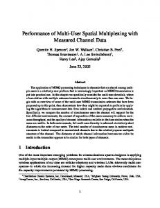
3. COMPARISION OF MIMO DETECTORS & CAPACITY MEASUREMENT Simulations are carried out under following Parameters & considerations. The channel experiences flat Raleigh fading, antennas are uncorrelated, perfect channel knowledge is available at the receiver, uniform power across transmit antennas, and there is independent Additive white Gaussian noise (AWGN) at each receiver. Here the experiments are performed based on MATLAB simulations of complex-valued 2×2 systems, averaging over random H with i.i.d. unit-variance complex circularly symmetric Gaussian entries. As measure of error performance of the minimum ratio of average received energy per bit (Eb) to one-sided noise power spectral density (N0) required to achieve a given bit error rate. Figure 1 give the points in the Bit error rate vs. Signal to Noise ratio (BER-SNR diagrams) for the following schemes: 1)
ZF detection.
2)
MMSE detection.
3)
ZF-SIC detection.
4)
MMSE-SIC detection.
5)
ZF-OSIC detection.
6)
MMSE-OSIC detection.
It can be seen that Non-linear schemes (SIC & OSIC) perform better than simple Linear detection schemes for both ZF as well as MMSE, and observe that MMSE detector outperforms ZF in all three categories because, the ZF cancel the interference completely at the expanse of enhancing of the Noise, where as MMSE minimize error due to noise and the interference combined. Among all sub-optimal detectors, particular the MMSE-OSIC provides best error performance. Since it has been known that Maximum Likelihood (ML) detector provides optimum performance but its computational complexity is increasing exponentially with increase in number of transmitting antennas, The MMSE-OSIC is better option for obtaining near-optimal performance with comparatively lesser complexity. The table 1 includes the required SNR values for various detector schemes at target BER of (10)-4. The detection complexity and the Diversity order for various detectors are also mentioned [11], [1].
Capacity for Multiple input multiple output (MIMO) with NT = n, NR = n is given by, 𝐶=
𝑟 𝐼=1 𝑙𝑜𝑔2 [1
2 + 𝜌/𝑛 𝑇 . 𝜒2𝑖 ]
(5)
7
International Journal of Computer Applications (0975 – 8887) Volume 125 – No.3, September 2015 BER VS SNR plot for SM detectors using 2*2 BPSK modulation in flat-fading channel
BER VS SNR plot for MMSE-OSIC using 2*2 8-QAM modulation in flat-fading channel theory (nTx=1,nRx=2, MRC) sim (nTx=2, nRx=2, ZF) sim (nTx=2, nRx=2, mmse) sim (nTx=2, nRx=2, zf-sic) sim (nTx=2, nRx=2, mmse-sic) sim (nTx=2, nRx=2, zf-osic) sim (nTx=2, nRx=2, mmse-osic)
-1
10
theory (nTx=1,nRx=2, MRC) sim (nTx=2, nRx=2, mmse-osic) 0
10
-1
10
-2
BER
10
-2
10
BER
-3
10
-3
10 -4
10
-4
10 -5
10
0
5
10
15
20 SNR(db)
25
30
35
40 -5
10
0
5
10
15
20
Fig 1: Comparison of Various SM Detectors with NR=NT=2
25 SNR(db)
30
35
40
45
50
Fig 3: BER v/s SNR Plot for MMSE-OSIC Detector using 8-QAM
Table 2. Comparison Table for Various SM Detection Schemes
BER VS SNR plot for MMSE-OSIC using 2*2 16-QAM modulation in flat-fading channel
No
Detector
SNR(db) at target BER (10)-4
theory (nTx=1,nRx=2, MRC) sim (nTx=2, nRx=2, mmse-osic)
Diversity Computational order complexity[9]
-1
10
-2
10
ZF
34
NR-NT+1
K to K
2
ZF-SIC
31.2
≈NRNT+1
K
3
ZFOSIC
BER
1
3
-3
10
-4
29.75
10
>NRNT+1NRNT+1