A Physical Model for Predicting Bidirectional ... - Science Direct

REMOTE SENS. ENVIRON. 27:273-288 (1989)

A Physical Model for Predicting Bidirectional Reflectances over Bare Soil Bernard Pinty * Michel M. Verstraete Robert E. Dickinson National Center for Atmospheric Research ~

R a d i a t i v e processes at the Earth's surface are affected by the soil optical properties. A good understanding of radiative transfer over a bare soil surface is therefore a prerequisite to addressing more complex cases of discontinuous vegetation canopies. While most attempts at retrieving surface characteristics are made by fitting empirical functions to the data, we have applied an optimization technique to a physically based surface reflectance model initially developed to study planetary surfaces. This inversion procedure allows the direct estimation of the following five parameters: the single scattering coefficient, two parameters describing the hot spot phenomenon, and two parameters describing the scattering phase function. The approach is validated by testing the inversion procedure against both synthetic data and actual observations. The model is able to predict the observed bidirectional reflectances, as

Address correspondence to Dr. Bernard Pinty, Natl. Ctr. for Atmos. Res., P.O. Box 3000, Boulder, CO 80307-3000 *Permanent affiliation: LAMP//OPGC, Universit~ Blaise Pascal, 63177 Aubibre, France. The National Center for Atmospheric Research is operated by the University Corporation for Atmospheric Research under the sponsorship ot the National Science Foundation. Received 25 August 1988; accepted 29 December 1988. 0034-4257/89/$3.50 ©Elsevier Science Publishing Co. Inc., 1989 655 Avenue o f the Americas, New York, NY 10010

well as the directional-hemispherical reflectances, and to build the complete field of radiances over the upward hemisphere. The anisotropic behavior of bare soils is investigated and the prospect for inferring other basic soil properties, such as the soil porosity, is discussed. INTRODUCTION Although the oceans cover some 71% of the surface of the Earth, the continents are responsible for much of the space and time variability of the climate system on time scales of 100 years or less. Land surface processes play an important role in this system by controlling the mass, momentum, and energy exchanges between the atmosphere and its lower boundary over continental areas (Verstraete and Dickinson, 1986). The atmosphere, in turn, affects the land surface through rock weathering, soil erosion, and constraints on biological activity. Under an atmosphere largely transparent to solar radiation, land areas provide a diversity of structure, composition, and spectral reflectance, and thereby affect the amount of solar radiation absorbed or reflected by the surface. By the same token, observations of the radiation scattered back

273

274 Pinty, Verstraete, and Dickinson

to space by the climate system can be interpreted physically in terms of atmospheric and surface properties. Because of their obvious importance, interactions between the atmosphere and the surface (and in particular the biosphere) have been studied at different scales and with tools of varying complexity. For example, the two-dimensional analytical model by' Anthes (1984), and the mesoscale simulations of Pinty et al. (1988) or Ookouchi et al. (1984) clearly show the dependency of the regional scale circulations on the nature and properties of the underlying surface. On an even larger scale, Dickinson and Henderson-Sellers (1988) show the complex effects of energy fluxes and their dependence on the nature and changes of surface properties in the Amazonian region. Other studies, prompted by the work of Charney (1975) and Otterman (1977), have shown the significant influence of surface albedo and soil moisture on the circulation of the atmosphere (e.g., Walker and Rowntree, 1977; or Sud and Fennessy, 1982). In this respect, satellite platforms appear to be the only means currently available to establish data bases compatible with mesoscale and global scale models. Such coherent data sets could provide adequate geographical coverage, continuous observation, and consistent accuracy. Furthermore, they may be analyzed and interpreted in terms of the physical, chemical, and biological properties of the surface needed by these models. Modeling and computer simulation need to be merged with the technology of satellite remote sensing (Thomas and Henderson-Sellers, 1987). For this purpose, inversion procedures must be performed with an accuracy of the retrieved parameters that is better than the maximum tolerable error in the model. The objective of the present paper is to develop a framework for using measurements of bidirectional reflectances to infer the anisotropy of the solar radiation reflected by land surfaces and to apply the method to a bare soil case. The bidirectional reflectances taken over the visible and near-infrared spectral ranges constitute one set of measurements currently available from satellites. There are basically two types of land information that can be retrieved from bidirectional reflectances: 1) the directional hemispherical reflectance (albedo), which controls the net radiative budget at the surface, and 2) land surface structure that directly or indirectly affects the sen-

sible and latent heat exchange with the atmospheric boundary layer, e.g., vegetation leaf area index, the percentage of ground cover, etc. Both of these types of information require the knowledge of the anisotropy of the radiance field. In the first case, the anisotropy, often expressed in terms of an anisotropy factor [defined below; see Eq. (4)], is required to properly derive the albedo of the surface (e.g., Koepke and Kriebel, 1987; Pinty and Ramond, 1987a). In the second case, the surface properties themselves can be extracted from an interpretation of the anisotropy of the medium with respect to light scattering (e.g., Goel and Thompson, 1984; Goel and Deering, 1985; Goel and Grier, 1987). Clearly, understanding the anisotropy of the surface should allow a better description of land surface processes and their impact on the climate system. Remote sensing in the visible and infrared spectral bands cannot acquire data below the soil surface, which therefore constitutes an effective lower boundary for the observed system. This soil surface may be significant at all scales larger than the local (micro) scale, either because the vegetation cover is discontinuous (Kimes et al., 1986) or because of the multiple scattering of radiation between the vegetation itself and the underlying soil surface. Thus a good understanding of the radiometric properties of soft surfaces is required before investigating vegetated surfaces, especially in the more complex case of discontinuous canopy Cover.

Several experiments have been conducted to quantify the anisotropy of bare soil surfaces. Remote sensing data at various scales, for example from the Nimbus 7 satellite (Taylor and Stowe, 1984) or from aircraft platforms (Salomonson and Marlatt, 1968), as well as field experiments (Eaton and Dirmhirn, 1979; Kimes et al., 1985; Walthall et al., 1985), all show that bare soil surfaces are highly anisotropic, with a preferential strong backscattering regime. Even over bright surfaces, such as sandy soils where multiple scattering is important and tends to lessen the anisotropy of the radiance field, directional effects are still observable (Salomonson and Marlatt, 1968). Relatively few attempts have been made to model the directional reflectance of bare soil surfaces (see, e.g., Egan and Hilgeman, 1978). Walthall et al. (1985) derived a functional representation with three parameters, namely the solar

Bare Soil Reflectance Model 275

zenith angle, the satellite viewing angle, and the relative azimuth angle, for the special case of rough surfaces. Other hmetions have been derived by Staylor and Suttles (1986) and Pinty and Ramond (19871)) to describe the anisotropic factors deduced from the Nimbus 7 ERB experiment over desertic regions of the globe. Although these functional fits are useful for providing a more realistic lower boundary condition than a Lambertian surface, none of these approaches results from or allows an adequate physical understanding of light scattering at the surface. It is therefore of great interest to note the comprehensive model developed by Hapke (1981; 1984; 1986) for the interpretation of radiometric properties of planetary surfaces. The bidirectional reflectance equation derived by Hapke relates the radiance field emerging from a surface to physically meaningful parameters such as the single scattering albedo, the particle phase hmction, the macroscopic slope, and the porosity of the surface. Hapke's model has been successfully applied to interpret reflectance measurements in the laboratory (Hapke and Wells, 1981), as well as those from various planetary surfaces (e.g., Hapke, 1984; Buratti, 1985; Helfenstein et al., 1988; Simonelli and Veverka, 1987). To our knowledge, no attempt has been made so far, however, to apply Hapke's model to investigate the reflectance of terrestrial bare soil surfaces. This study examines how well the bidirectional reflectance fields measured over bare softs can be predicted by Hapke's model. After a brief description of the bidirectional reflectance equation derived by Hapke, we describe the approach used for fitting this equation to experimental data. This approach, based on a nonlinear least square fitting of the equation, is commonly used to infer several parameters from bidirectional remote sensing measurements. A simulation study, using model-generated data, has been conducted before applying the theory to the field data, as was done by Camftlo (1987).

DESCRIPTION

OF

HAPKE'S M O D E L

Starting from the fundamental principles of radiative transfer theory, Hapke (1981) derived an analytical equation for the bidirectional reflectance function of a medium composed of particles. The

singly scattered radiance is computed exactly, whereas the multiply scattered radiance is evaluated from a two-stream approximation, assuming that the scatterers making up the surface are isotropic. The bidirectional reflectance r of a surface illuminated with a solar zenith angle i, viewed from a zenith angle e, and normalized with respect to the reflectance of a perfectly reflecting Lambertian surface under the same conditions of illumination and observation, is given by w

1

([1+ B ( g ) ] P ( g )

r(i,e,~)--- 4 c o s i + c o s e + H(cosi)n(cose)- 1}, (1) where cos g = cos i cos e + sin i sin e cos ~b, Bo B(g)= [l+(1/h)tan(g/2)]'

s(0) B° = ~0P(0) '

e(g)-- 1 + bcosg + c[(3cos2g- 1)/2], {

(l+2x))

In Eq. (1-), ~ is the viewing azimuth relative to the Sun's azimuth, g is the phase angle between the incoming and the outgoing rays, o~ is the average single scattering albedo of the particles making up the surface, P(g) is the average phase function as approximated by a second-order Legendre polynomial expansion, B(g) is a backscattering function that accounts for the opposition effect arising at low phase angle, and the term H(cos i)H(cos e) - 1 approximates the contribution from multiple scattering. Although some numerical calculations of bidirectional reflectances with a canopy model (Kimes, 1984) suggest that this approximation can be rather inaccurate, Hapke's approximation is followed here. In addition to w, there are basically four unknown parameters in this equation: b and c, S(0), and h. The parameters b and c are the coefficients of the Legendre polynomial expansion used to express the particle phase function. The dominant scattering regime can also be expressed in terms of the asymmetry factor O = (cos(~r - g)) = - 5/3. Negative values of O indicate preferential backscattering, while positive ones represent for-

276 Pinty, Verstraete,and Dickinson ward scattering. The term S(O) corresponds to the amplitude of the opposition surge, i.e., the preferential escape of radiation for viewing direction close to that of the Sun, and h characterizes the width of this opposition surge and may be related to the grain size distribution, the porosity, and the gradient of compaction with depth. This opposition effect (also called hot spot) is often observed on various surfaces (Kriebel, 1978; Walthall et al., 1985; Ranson et al., 1985) and, according to Hapke, is caused by the hiding of shadows at low phase angles. Equation (1) includes the improved formulation for B(g) (Hapke, 1986) instead of the original expression given in Hapke (1981), but it neglects the macroscopic roughness effect discussed Hapke (1984). The inclusion of this latter effect would increase to six the total number of unknown parameters in the model.

APPLICATION OF THE MODEL The basic problem of remote sensing is the interpretation of the data in terms of the physical quantities of interest for the observed surface. If the radiometric properties of a bare soil surface can indeed be described by Eq. (1), the interpretation problem consists in finding the values of the five parameters ~0, S(0), h, b, and c such that the computed value of r best approximates the actual observations in some sense. In this study, we adopted a nonlinear least square fitting procedure. We define a quantity

82= ~ [rk--r(ik,ek,gk)] 2,

(2)

ables, using function values only. Since it requires an initial guess for each of the desired parameters, we have also established the sensitivity of the results to the selection of this initial guess.

Synthetic Data In order to test the applicability and accuracy of this procedure, a number of experiments were performed using bidirectional reflectances data generated with Eq. (1). Two basic sets of data were built, denoted A and B, to represent possible variations of the five parameters to investigate. For data set A, ~ = 0.1, S(0) = 0.2, h = 0.1, b = - 0.5, and c = 0, and the corresponding values for data set B are 0~ = 0.8, S(0) = 2.0, h = 0.6, b = 0.5, and c = 0. These values will be referred to as "true values" later. In both cases, a total of 60 bidirectional reflectance values were generated. These were computed for two values of the solar zenith angle, i = 30 ° and 50 °, with, in each case, the viewing angle e varying from 0 ° to 75 ° in increments of 15 °, and with the relative azimuth angle tp varying from 0 ° to 180 ° in increments of 45 °. This particular sampling of the bidirectional reflectance field has been chosen to closely match that of the actual data set used in the next section. As a first step, we conducted tests with these two data sets (A and B), to investigate the performance of the procedure under ideal conditions. In a second step, we perturbed these "clean" data with random noise to investigate to what extent one could retrieve the "true values" even with "noisy" data.

k=l

where rk is the measured bidirectional reflectance of the surface for the relative geometry of illumination and observation defined by i k, e k, gk, and r is the modeled bidirectional reflectance. If the measured values are not uniformly distributed, appropriate weights could be introduced in Eq. (2). The problem then reduces to finding the optimal values of these five parameters which minimize 89. for a given set of actual observations. The routine E04JAF from the Numerical Algorithms Group (NAG) library was chosen for this purpose. This routine implements a quasi-Newton algorithm for finding a minimum of a function, subject to fixed upper and lower bounds on the independent vari-

Clean Data Set We applied the optimization procedure described above to establish to what extent we could retrieve the "true values" of the parameters of Eq. (1) using data sets of known characteristics. This was done for both data sets A and B, once with an initial guess equal to the true values used for generating the data, and once with an arbitrary initial guess somewhere in between the parameter values of data sets A and B. From the results shown in Table 1, it appears that the retrieved values are not very sensitive to the initial guess. The column titled "RMS" gives the value of the root mean square of the fit, i.e., ~82/Nf, where Nr

Bare Soil Reflectance Model 277

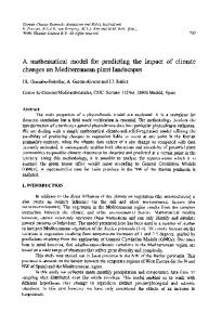
leads to better estimates for all five parameters (Table 2). In the second test, the illumination angle sampling frequency was increased from one solar position at 30 ° to six solar positions, from 30 ° to 80 °, in increments of 10 °. In this case, the values retrieved by the optimization procedure converge to the true values for data set A (Fig. 1). Hence, as expected, the accuracy of the inversion procedure increases with finer resolution of sampiing in solar and viewing angles.

is the number of degrees of freedom, which is the number of independent data points minus the number of parameters estimated by the procedure. This RMS value is not zero for a number of reasons including the intrinsic limitations of the quasi-Newton algorithm as implemented by routine E04JAF, the accuracy of the computations, and the frequency of sampling of the original function. The impact of the frequency of sampling on the quality of the inversion procedure was examined by looking at the difference between the true values and the values of the five retrieved parameters, in the ideal case where the initial guess was equal to these true values. This was performed first by increasing the observing angle sampling frequency of data sets A and B. This higher observing frequency was achieved by generating data in increments of 10 ° in viewing angle and 30 ° in relative azimuth angle; such a data set has about twice the angular resolution of the original data sets A and B. The higher observing frequency

Noisy Data Set In "real-life" situations, the observational data are contaminated by noise due to the physical characteristics of the instrument, and the conditions of observation. The question then arises as to whether the optimization procedure would also be capable of retrieving the correct values of the parameters even if the data were noisy, or, in other words, what is the maximum amount of random noise that can be tolerated in the data before the retrieved

Table 1. Clean Data S(O)

h

b

c

RMS o f fit

- 0.500 - 0.500 - 0.452 0.000 - 0.447

0.0000 0.0000 0.0093 0.0000 - 0.0089

2.9 x 10 4

0.500 0.500 0.501 0.000 0.501

0.0000 0.0000 0.0015 0.0000 0.0015

3.0 X 10 4

Set A T r u e value Initial guess R e t r i e v e d value Initial guess R e t r i e v e d value

0.100 0.100 0.105 0.500 0.106

0,200 0,200 0.193 0.500 0.192

0.100 0.100 0.091 0.200 0.089

T r u e value Initial guess R e t r i e v e d value Initial guess Retrieved value

0.800 0.800 0.801 0.500 0.801

2,000 2.000 1.991 0.500 1.991

0.600 0.600 0.598 0,200 0.598

2.9 x 10 4

Set B

Table 2.

Effect of the Observing

Sampling Frequency

3.1 × 10 4

on the Retrieved Values

S(0)

h

b

c

Set A True value I.O.S.F. a E.O.S.F. b

0.100 - 5.1599 x 1 0 - 3 -4.0726x10 -3

0,200 7.2639 x 1 0 - 3 5.0050x10 3

True value I.O.S.F. a E.O.S.F. b

0.800 - 1.0316 x 10 - 3 - 1.4241 x 10 - 4

2.000 9.1293 x 10 - 3 3.3718 x 10 - 3

0,100 9.2408 X 10 3 6.5684X10 3

- 0,500 4.8245 x 1 0 - 2 3.1911x10 2

0.0000 - 0.9327 x 1 0 - 2 -0.4524x10 2

0.500 - 1.0706 X I0 - 3 4.5470 X 10 5

0.0000 0.1493 x 10 2 0.1317 X 10 2

Set B 0.600 1.7949 X 10 - 3 - 2.8252 X 10 3

a I . O . S . F . = t r u e values m i n u s r e t r i e v e d values for the Initial O b s e r v a t i o n S a m p l i n g F r e q u e n c y . b E . O . S . F . = t r u e values m i n u s r e t r i e v e d values for the E n h a n c e d O b s e r v a t i o n S a m p l i n g F r e q u e n c y .

278 Pintg, Verstraete, and Dickinson

10.0 m -s

8.0

-6

6.0

i

2± ....

-l- -

~ s(o)

I .

~

i

,

..h

4.0 .

o>

2.0

o

0.0

k_

•k..

-2.0

,

-4.0

m

-6.0

x._ I--

-8.0

.

.

.

.

.

Angular sampling frequency

Figure I. Evolution of the difference b e t w e e n the true values of t h e five p a r a m e t e r s minus the retrieved values, as a f u n c t i o n of the sampling f r e q u e n c y in solar z e n i t h angle, for data set A. T h e n u m b e r in abscissa i n d i c a t e s t h e n u m b e r of solar zenith angles available for t h e retrieval process, to, S(0), and h in units of 10 3 a n d b a n d c in units of 10-2.

parameters become unacceptably different from their true values. To address this question, we added some random noise (of zero mean and known variance) to each value of the data sets A and B described above, and repeated this operation 500 times. In

other words, we generated 500 data sets of 60 reflectance values each, which were then inverted using the procedure described above [Eq. (2)]. The results averaged over these 500 data sets are shown in Table 3. With noisy data, the optimization procedure cannot always find an unambiguous

cJ

-10.0

r

f

I

i

I

I

1

2

5

5

4

5

Table 3. Noisy D a t a S.D."

~o

S(O)

h

b

c

True value Initial guess Retrieved value (Stand. dev.) Initial guess Retrieved value (Stand. dev.) Initial guess Retrieved value (Stand. dev.) Initial guess Retrieved value

0.100 0.100 0.094 (0.038) 0.500 0.096 (0.036) 0.100 0.093 (0.040) 0.500 0.096

0.200 0.200 0.197 (0.047) 0.500 0.197 (0.046) 0.200 0.208 (0.076) 0.500 0.207

0.100 0.100 0.095 (0.073) 0.200 0.089 (0.066) 0.100 0.I03 (0.115) 0.200 0.124

- 0.500 - 0.500 - 0.515 (0.235) 0.000 - 0.509 (0.223) - 0.500 0.519 (0.290) 0.000 - 0.545

0.000 0.000 - 0.064 (0.111) 0.000 - 0.062 (0.107) 0.000 - 0.074 (0.198) 0.000 - 0.090

(Stand. dev.)

(0.046)

(0.081)

(0.159)

(0.272)

(0.218)

True value Initial guess Retrieved value (Stand. dev.) Initial guess Retrieved value

0.800 0.800 0.794 (0.045) 0.500 0.794

2.000 2.000 2.023 (0.446) 0.500 2.023

Set B 0.600

0.500

0.000

0.600

0.500

0.000

0.653

0.514

0.002

(Stand. dev.) Initial guess Retrieved value (Stand. dev.) Initial guess Retrieved value (Stand. dev.)

(0.045) 0.800 0.775 (0.102) 0.500 0.775 (0.102)

(0.446) 2.000 2.120 (0.840) 0.500 2.130 (0.840)

(0.262) 0.200 0.652 (0.262) 0.600 0.640 (0.339) 0.200

(0.177) 0.000 0.515 (0.177) 0.500 0.521 (0.315) 0.000

(0.134) 0.000 0.002 (0.133) 0.000 0.006 (0.252) 0.000

0.630

0.521

0.005

(0.339)

(0.315)

(0.253)

Nb

RMS o f fit

417

0.005

369

0.005

375

O.OlO

291

0.010

500

0.05

498

0.05

493

0.10

490

0.10

Set A 0.005

0.005

0.010

0.010

0.05

0.05

0.10

0.10

~S.D. = standard deviation of the input data. bN = number of successhd cases, out of 500.

Bare Soil Reflectance Model

minimum, and the computer routine issues a message to the effect that the value found may not be optimal. These cases were discarded altogether. The column entitled N shows the number of cases in which the optimization procedure actually found a minimum. If such a situation of nonconvergence were encountered in fitting observational data, some alternative procedure would be required, e.g., a separate fitting of the opposition effect parameters using only viewing angle data in the direction of the Sun, or some manual selection of the parameters to be fitted. For each data set A and B, two values of the standard deviation of the noise, corresponding approximately to 5 and 10% of the bidirectional reflectance values, were used. Here again, the inversion procedure was initialized with two guesses, one being the true values and the other the intermediate values given earlier. The root-mean-square (RMS) value for the fit is equal (within rounding-off errors) to the standard deviation of the noise added to the data, since the "noise" inherent to the optimization procedure is an order of magnitude lower than this external noise, as shown in Table 1. By and large, the inversion procedure worked better for data set B, with a larger single scattering albedo value, than for data set A, in the sense that, for set B, the standard deviations of the retrieved values represent smaller fractions of the average values. Furthermore, the sensitivity to the values of the initial guess is smaller for data set B than for data set A. The optimization procedure was also able to find a satisfactory minimum more often for this data set than data set A. The characteristics of the optimization procedure can be quantified by performing statistical tests on the data, since the average and variance of the initial noise distribution are known a pr/or/, and the mean and standard deviation of the results are given. From statistical decision theory (e.g., Hoel, 1971), it is known that, for uncorrelated errors, 95% of the time ~,

s

cases, because of the large number of cases. In that table, the underlined values are those such that the actual mean does not fall within this interval at the 95% level. It therefore appears that, for the angular sampling frequency used here, the optimization procedure described above may introduce a bias in the estimation of the physical parameters of the surface. This issue will be considered in a forthcoming paper.

Field Data We now apply this inversion procedure by optimization to actual field data. Few data sets are detailed enough to allow a rigorous test. We used the field data gathered by Kimes et al. (1985) over a plowed field. These data were taken at 2 m above the ground, with a radiometer operating in the same bands as the NOAA 7 / 8 satellite AVHRR (Band 1 = 0.58-0.68 ~tm, and Band 2 = 0.73-1.1 /~m). The bidirectional reflectances were sampled each 45 ° in azimuth between 0 ° and 180 °, and each 15 ° in zenith viewing angle between 0 ° and 75 °. A total of 30 measurements are therefore available for each solar zenith angle. The radiances at each sampled angle were further normalized by the radiances from a Lambertian refector illuminated under the same conditions. Assuming 1) that the studied surface is horizontal and uniform over a domain area large with respect to the size of the sampled area (so that boundary effects can be neglected) and 2) that the measured bidirectional refiectances are taken just above the surface (so that the extinction of the radiation by the atmosphere between the surface and the sensor is negligible), one can express the measured bidirectional reflectances R as follows: R(i,e,+)=r(i,e,q~) +[r(i,e,+)-r(i,e,+)]fa(i),

where

e,,(i) Et(i)'

s

--t0'975~