Hindawi Publishing Corporation Mathematical Problems in Engineering Volume 2014, Article ID 627416, 10 pages http://dx.doi.org/10.1155/2014/627416
Research Article A Plant Propagation Algorithm for Constrained Engineering Optimisation Problems Muhammad Sulaiman,1,2 Abdellah Salhi,1 Birsen Irem Selamoglu,1 and Omar Bahaaldin Kirikchi1 1 2
Department of Mathematical Sciences, University of Essex, Colchester CO4 3SQ, UK Department of Mathematics, Abdul Wali Khan University, Mardan KPK, Pakistan
Correspondence should be addressed to Muhammad Sulaiman;
[email protected] Received 17 February 2014; Accepted 6 April 2014; Published 7 May 2014 Academic Editor: Changzhi Wu Copyright © 2014 Muhammad Sulaiman et al. This is an open access article distributed under the Creative Commons Attribution License, which permits unrestricted use, distribution, and reproduction in any medium, provided the original work is properly cited. Optimisation problems arising in industry are some of the hardest, often because of the tight specifications of the products involved. They are almost invariably constrained and they involve highly nonlinear, and non-convex functions both in the objective and in the constraints. It is also often the case that the solutions required must be of high quality and obtained in realistic times. Although there are already a number of well performing optimisation algorithms for such problems, here we consider the novel Plant Propagation Algorithm (PPA) which on continuous problems seems to be very competitive. It is presented in a modified form to handle a selection of problems of interest. Comparative results obtained with PPA and state-of-the-art optimisation algorithms of the Natureinspired type are presented and discussed. On this selection of problems, PPA is found to be as good as and in some cases superior to these algorithms.
1. Introduction Optimisation problems in design engineering are often highly nonlinear, constrained and involving continuous as well as discrete variables [1–5]. It is also often the case that some of the constraints are active at the global optimum [6]. This means that feasible approximate solutions are that much harder to find. There is a variety of algorithms for these problems, some exact, and others approximate. In the exact category, one can name Branch-and-Bound, [7], Recursive Quadratic Programming, [8], the Cutting Plane Algorithm [9], Bender’s decomposition [10]. Of the approximate variety, one can name Simulated Annealing, [11–13], the Genetic Algorithm [14–16], and the Particle Swarm Optimisation algorithm, [17, 18], to name a few. The latter category is often referred to as the metaheuristic algorithms. In general, they are characterised by two aspects
of the search: exploration of the overall search space and exploitation of good areas in order to find local optima, [19–22]. A new metaheuristic, the Plant Propagation Algorithm (PPA), has recently been introduced [23]. PPA is nature inspired [19, 23, 24]; it emulates the way plants, in particular the strawberry plant, propagate. A basic PPA has been described and tested on single objective as well as multiobjective continuous optimization problems in [23]. The test problems, though standard, were of low dimension. The results showed that PPA has merits and deserves further investigation on higher dimensional problem instances as well as problems arising in practice, for these are often very challenging. PPA is attractive because, among other things, it is simple to describe and implement; it also involves only few parameters that need arbitrary setting unlike most other metaheuristics. Here, it will be tested on constrained
2
Mathematical Problems in Engineering
optimisation problems arising in engineering. The paper is organised as follows. Section 2 describes PPA. Section 3 presents a modified version to handle constrained problems. Section 4 records the results obtained with PPA and a number of other heuristics. In Section 5 a conclusion and ideas for further investigation are given. The paper includes appendices that describe the problems considered.
2. The Strawberry Algorithm as PPA The Strawberry algorithm is an exemplar PPA which can be seen as a multipath following algorithm unlike Simulated Annealing (SA) [13, 25], for instance, which is a single path following algorithm. It can, therefore, be perceived as a generalisation of SA and other path-following algorithms [26]. Exploration and exploitation are properties that effective global optimisation algorithms have [19, 24, 26]. Exploration refers to the property of covering the search space, while exploitation refers to the property of searching nearer to good solutions for local optima. Consider what a strawberry plant and possibly any plant which propagates through runners will do to optimize its survival. If it is in a good spot of the ground, with enough water, nutrients, and light, then it is reasonable to assume that there is no pressure on it to leave that spot to guarantee its survival. So, it will send many short runners that will give new strawberry plants and occupy the neighbourhood as best they can. If, on the other hand, the mother plant is in a spot that is poor in water, nutrients, light, or any one of these necessary for a plant to survive, then it will try to find a better spot for its offspring. Therefore, it will send few runners further afield to explore distant neighbourhoods. One can also assume that it will send only a few, since sending a long runner is a big investment for a plant which is in a poor spot. We may further assume that the quality of the spot (abundance of nutrients, water, and light) is reflected in the growth of the plant. With this in mind and the following notation, PPA can be described as follows. A plant 𝑝𝑖 is in spot 𝑋𝑖 in dimension 𝑛. This means 𝑋𝑖 = {𝑥𝑖,𝑗 , for 𝑗 = 1, . . . , 𝑛}. Let 𝑁𝑃 be the number of strawberry plants to be used initially, and the PPA algorithm described in pseudo-code Algorithm 1, relies on the following strategy [23]. (i) Strawberry plants which are in good spots propagate by generating many short runners. (ii) Those in poor spots propagate by generating few long runners. It is clear that, in the above description, exploitation is implemented by sending many short runners by plants in good spots, while exploration is implemented by sending few long runners by plants in poor spots. The parameters used in PPA are the population size 𝑁𝑃 which is the number of strawberry plants, the maximum number of generations 𝑔max , and the maximum number of possible runners 𝑛max per plant. 𝑔max is effectively the stopping criterion in this initial version of PPA. The algorithm
uses the objective function value at different plant positions 𝑋𝑖 , 𝑖 = 1, . . . , 𝑁𝑃, in a normalised form 𝑁𝑖 , to rank them as would a fitness function in a standard genetic algorithm (note that, unlike in the GA, individuals in PPA are clones of the mother plant; they do not improve from generation to generation). The number of plant runners 𝑛𝛼𝑖 , calculated according to (1) below, has length 𝑑𝑥𝑖 calculated using the normalised form of the objective value at 𝑋𝑖 , each giving a 𝑑𝑥𝑖 ∈ (−1, 1)𝑛 , as calculated with (2) below. After all individuals/plants in the population have sent out their allocated runners, new plants are evaluated and the whole increased population is sorted. To keep the population constant, individuals with lower growth are eliminated. The number of runners allocated to a given plant is proportional to its fitness as in 𝑛𝛼𝑖 = ⌈𝑛max 𝑁𝑖 𝛼⌉ ,
𝛼 ∈ (0, 1) .
(1)
Every solution 𝑋𝑖 generates at least one runner and the length of each such runner is inversely proportional to its growth as in (2) below: 𝑑𝑥𝑗𝑖 = 2 (1 − 𝑁𝑖 ) (𝛼 − 0.5) ,
for 𝑗 = 1, . . . , 𝑛,
(2)
where 𝑛 is the problem dimension. Having calculated 𝑑𝑥𝑖 , the extent to which the runner will reach, the search equation that finds the next neighbourhood to explore is 𝑦𝑖,𝑗 = 𝑥𝑖,𝑗 + (𝑏𝑗 − 𝑎𝑗 ) 𝑑𝑥𝑗𝑖 ,
for 𝑗 = 1, . . . , 𝑛.
(3)
If the bounds of the search domain are violated, the point is adjusted to be within the domain [𝑎𝑗 , 𝑏𝑗 ], where 𝑎𝑗 and 𝑏𝑗 are lower and upper bounds delimiting the search space for the 𝑗th coordinate.
3. An Effective Implementation of PPA for Constrained Optimization In this implementation of PPA, the initial population is crucial; we run the algorithm a number of times from randomly generated populations. The best individual from each run forms a member of the initial population. The number of runs to generate the initial population is 𝑁𝑃; therefore, the population size is 𝑟 = 𝑁𝑃. In the case of mixed integer problems, the integer variable values are fixed when they are showing a trend to converge to some values. This trend is monitored by calculating the number of times their values have not changed. When this number is greater than a certain threshold, the variables are fixed for the rest of the run. This strategy seems to work on the problems considered. Let 𝑝𝑜𝑝 be a general matrix containing the population of a given run. Its rows correspond to individuals. The following equation is used to generate a random population for each of the initial runs: 𝑥𝑖,𝑗 = 𝑎𝑗 + (𝑏𝑗 − 𝑎𝑗 ) 𝛼,
𝑗 = 1, . . . , 𝑛,
(4)
where 𝑥𝑖,𝑗 ∈ [𝑎𝑗 , 𝑏𝑗 ] is the 𝑗th entry of solution 𝑋𝑖 and 𝑎𝑗 and 𝑏𝑗 are the 𝑗th entries of the lower and upper bounds describing the search space of the problem and 𝛼 ∈ (0, 1).
Mathematical Problems in Engineering
3
∗ = 𝑥𝑖,𝑗 (1 + 𝛽) , 𝑥𝑖,𝑗
𝑗 = 1, . . . , 𝑛,
(5)
8500 8000
𝑗 = 1, . . . , 𝑛,
5500
0
(7)
∗ ∈ [𝑎𝑗 , 𝑏𝑗 ], and 𝑘 is different from 𝑖. To where 𝛽 ∈ [−1, 1], 𝑥𝑖,𝑗 keep the size of the population constant, the extra plants at the bottom of the sorted population are eliminated.
20
40
60
80
Pm = 0.8 Pm = 1.0
Pm = 0.1 Pm = 0.6
Figure 1: Impact of the particular probability 𝑃𝑚 on the performance of PPA. 15 10 5 0
−5 −10 −15
Step size decreases as the population converges during each run. This helps PPA to exploit the solution space 0
0.5
1
1.5
Perturbations produced by rules 2-3
4. Examples of Structural Engineering Optimization Problems PPA as explained in the pseudo-code Algorithm 1 is extended to cater for constrained optimisation problems to be found in the appendices [6, 27]. This extended version of PPA is fully explained in the pseudo-code Algorithm 2. Note that the penalty function approach is used to handle the constraints [19, 22]. Equations are first transformed into inequality constraints before they are taken into consideration. Table 1 records the parameter values used in the implementation. Column 4 shows the value of 𝑃𝑚 used throughout the experiments. This value has been found through experimentation on the problem described in Appendix B. The different runs are represented in Figure 1 where for 40 trials corresponding to the 30000 function evaluations threshold, 𝑃𝑚 = 0.8 seems to be the optimal value for this parameter. Other aspects of the extended algorithm such as exploration and exploitation are investigated in Figures 2 and 3. These figures, as one expects, show that the magnitudes of the steps/perturbations of the plant positions, that is the lengths of the runners,
100
Number of trial runs
(6)
∗ where 𝛽 ∈ [−1, 1], 𝑥𝑖,𝑗 ∈ [𝑎𝑗 , 𝑏𝑗 ]. 𝑙, 𝑘 are mutually exclusive indices and are different from 𝑖. The generated individual 𝑋𝑖∗ is evaluated according to the objective function and is stored in Φ. The first two rules are applicable for 𝑟 ≤ 𝑁𝑃 the number of runs. For 𝑟 > 𝑁𝑃 the algorithm also tries to recognise entries which are settling to their final values through a counter 𝐼𝑁. If the 𝑗th entry in current population has a low 𝐼𝑁 value, then it is modified by implementing (7); otherwise it is left as it is. The value (for 𝐼𝑁) that is suggested by experimentation over a number of problems is 4. The following equation is used when modification is necessary: ∗ = 𝑥𝑖,𝑗 + (𝑥𝑖,𝑗 − 𝑥𝑘,𝑗 ) 𝛽, 𝑥𝑖,𝑗
Better convergence rate at Pm = 0.8 and Pm = 1.0
7000
6000
Search space limits
𝑗 = 1, . . . , 𝑛,
7500
6500
∗ where 𝛽 ∈ [−1, 1] and 𝑥𝑖,𝑗 ∈ [𝑎𝑗 , 𝑏𝑗 ]. The generated individual 𝑋𝑖∗ is evaluated according to the objective function and is stored in Φ. In rule 02 another individual is created with the same modification parameter 𝑃𝑚 = 0.8 as in the following equation: ∗ 𝑥𝑖,𝑗 = 𝑥𝑖,𝑗 + (𝑥𝑙,𝑗 − 𝑥𝑘,𝑗 ) 𝛽,
Pressure vessel design
9000
Objective values
In the main body of the algorithm, before updating the population we create a temporary population Φ to hold new solutions generated from each individual in the population. Then we implement three rules with fixed modification parameter 𝑃𝑚 , chosen here, as 𝑃𝑚 = 0.8. The first two rules are implemented if the population is initialized randomly. Rule 01 uses the following equation to update the population:
2
2.5
×106
Figure 2: Exploitation characteristic of PPA using rules 2-3.
get shorter and shorter as the search progresses. Figure 4 is a representation of the convergence of the objective values of the problems described in Appendices A and C. In both cases, these values fluctuate wildly before they settle down to very good approximate values. The numerical results of the experiments on all problems described in Appendices A, through G are compiled in Tables 2, 3, 4, 5, 6, 7, and 8.
5. Conclusion We have implemented PPA to solve seven well known difficult constrained optimization problems arising in engineering design with continuous domains. PPA found either near best known solutions or optimal ones to all of them. The results are compared to those obtained with other algorithms found in the literature, namely GA (and variants of it, here denoted EC and EP), PSO, HSA (and variants of it
4
Mathematical Problems in Engineering
Table 1: Parameters used in PPA for seven engineering problems. Problem Welded beam Pressure vessel Spring design Speed reducer Constrained Problem I Constrained Problem II Himmelblau’s function
Population size 40 40 40 40 40 40 40
𝑃𝑚 0.8 0.8 0.8 0.8 0.8 0.8 0.8
Maximum iteration 20 20 25 20 20 20 25
Max function evaluations 30000 30000 30000 30000 24000 24000 30000
Number of runners 3 3 3 3 3 3 3
Runs 100 100 100 100 100 100 100
Table 2: Welded beam design optimisation. Solution vector GA [28] 𝑤 0.2088 𝐿 3.4205 𝑑 8.9975 ℎ 0.2100 −0.3378 𝑔1 (𝑥) −353.9026 𝑔2 (𝑥) −0.0012 𝑔3 (𝑥) −3.4118 𝑔4 (𝑥) −0.0838 𝑔5 (𝑥) −0.2356 𝑔6 (𝑥) −363.2323 𝑔7 (𝑥) 𝑓(𝑥) 1.7483 a
HSA [29] 0.2442 6.2231 8.2915 0.2443 ∗a ∗ ∗ ∗ ∗ ∗ ∗ 2.38
HSA [30] 0.2057 3.4704 9.0366 0.2057 ∗ ∗ ∗ ∗ ∗ ∗ ∗ 1.7248
HHSA [31] 0.2057 3.4706 9.0368 0.2057 ∗ ∗ ∗ ∗ ∗ ∗ ∗ 1.7248
BDA [32] 0.2057 3.4704 9.0366 0.2057 0.0 0.0 −5.5511𝐸 − 17 −3.4329 −0.0807 −0.2355 −9.0949𝐸 − 13 1.7248
PHS [27] 0.2057 3.4704 9.0366 0.2057 0.0 0.0 −5.5511𝐸 − 17 −3.4329 −0.0807 −0.2355 −9.0949𝐸 − 13 1.7248
IPHS [27] 0.2057 3.4704 9.0366 0.2057 0.0 0.0 −5.55𝐸 − 17 −3.4329 −0.0807 −0.2355 −9.09𝐸 − 13 1.7248
PPA 0.2057 3.4704 9.0366 0.2057 −1.2733𝐸 − 11 −3.2378𝐸 − 11 −1.64𝐸 − 13 −3.4329 −0.0807 −0.2355 −6.2755𝐸 − 11 1.7248
IPHS [27] 1.125 0.625 58.2901 43.6927 −3.3595𝐸 − 7 −0.0689 −0.0705 −196.307 7197.730
PPA 0.7781 0.3846 40.3196 200.0 3.627𝐸 − 12 1.441𝐸 − 12 1.1641𝐸 − 9 −40.0 5885.3327
IPHS [27] 0.0518 0.3608 11.0503 −2.1962𝐸 − 6 −2.8408𝐸 − 7 −4.0618 −0.7248 0.01266
PPA 0.0515 0.3541 11.4387 −5𝐸 − 15 −1.3901𝐸 − 9 −4.0487 −0.7294 0.01266
Not available.
Table 3: Pressure vessel design optimisation. Solution vector 𝑑1 𝑑2 𝑟 𝐿 𝑔1 (𝑥) 𝑔2 (𝑥) 𝑔3 (𝑥) 𝑔4 (𝑥) 𝑓(𝑥)
IP(M-5) [7] 1.125 0.625 48.97 106.72 −0.1799 −0.1578 −97.760 −133.28 7980.894
GA [14] 1.125 0.625 58.1978 44.2930 0.0017 −0.0697 −974.3 −195.707 7207.494
HSA [29] 1.125 0.625 58.2789 43.7549 −0.0002 −0.0690 −3.7162 −196.245 7198.433
HSA [30] 1.125 0.625 58.2901 43.6926 0.0000 −0.0689 −2.0150 −196.307 7197.730
PHS [27] 1.125 0.625 58.2874 43.7075 −5.2058𝐸 − 005 −0.0689 −0.6122 −196.29 7197.896
Table 4: Minimization of the weight of a compression spring. Solution vector 𝑥1 𝑥2 𝑥3 𝑔1 (𝑥) 𝑔2 (𝑥) 𝑔3 (𝑥) 𝑔4 (𝑥) 𝑓(𝑥)
MP(M-5) [33] 0.0500 0.3159 14.2500 −0.00001 −0.0037 −3.9383 −0.7560 0.01283
EC [34] 0.0533 0.3991 9.1854 0.00001 −0.00001 −4.1238 −0.6982 0.01273
GA [28] 0.0519 0.3639 10.8905 −0.00001 −0.00002 −4.0613 −0.7226 0.01268
BDAs [32] 0.0514 0.3513 11.6086 −0.0033 −1.0970𝐸 − 4 −4.0263 −0.7312 0.01266
PHS [27] 0.0500 0.3173 14.0375 −4.7653𝐸 − 6 −1.8124𝐸 − 4 −3.9672 −0.7550 0.01272
Mathematical Problems in Engineering
5 Table 5: Speed reducer design optimisation.
Solution vector 𝑥1 𝑥2 𝑥3 𝑥4 𝑥5 𝑥6 𝑥7 𝑔1 (𝑥) 𝑔2 (𝑥) 𝑔3 (𝑥) 𝑔4 (𝑥) 𝑔5 (𝑥) 𝑔6 (𝑥) 𝑔7 (𝑥) 𝑔8 (𝑥) 𝑔9 (𝑥) 𝑔10 (𝑥) 𝑔11 (𝑥) 𝑓(𝑥) a
PSO [6] 3.50 0.70 17.0 7.30 7.80 3.3502 5.2866 −0.0739 −0.1979 −0.4991 −0.9014 0.0000 −5.000𝐸 − 16 −0.7025 −1.000𝐸 − 16 −0.5833 −0.0513 −0.0108 2,996.3481
AAI [35] 3.50 0.70 17.0 7.30 7.71 3.35 5.29 ∗a ∗ ∗ ∗ ∗ ∗ ∗ ∗ ∗ ∗ ∗ 2994.4
PHS [27] 3.50 0.70 17.0 7.30 7.7159 3.3502 5.2869 ∗ ∗ ∗ ∗ ∗ ∗ ∗ ∗ ∗ ∗ ∗ 2994.9
PPA [𝜇 = 𝐸5.488] 3.4922 0.70 17.0 7.30 7.80 3.3496 5.2846 −0.07185 −0.1962 −0.4988 −0.9013 4.6229𝐸 − 4 1.816𝐸 − 3 −0.70250 2.2248𝐸 − 3 −0.5842 −0.0514 −0.01114 2994.4449
IPHS [27] 3.50 0.70 17.0 7.30 7.7153 3.3502 5.2866 ∗ ∗ ∗ ∗ ∗ ∗ ∗ ∗ ∗ ∗ ∗ 2994.4
PPA [𝜇 = 𝐸5.93101] 3.4971 0.70 17.0 7.30 7.80 3.3500 5.2866 −0.07317 −0.1973 −0.4990 −0.9014 1.667𝐸 − 4 6.564𝐸 − 4 −0.7025 8.0440𝐸 − 4 −0.58366 −0.05136 −0.0108 2996.1137
Not available.
Table 6: Constrained optimization problem I.
×105 9
GAs [36] 0.8080 0.8854 3.7𝐸 − 2 5.2𝐸 − 2 1.4339
EP [37] 0.8350 0.9125 1𝐸 − 2 −7𝐸 − 2 2.3772
HSA [29] 0.8343 0.9121 5𝐸 − 3 5.4𝐸 − 3 1.3770
PHS [27] 0.8230 0.9113 1.1880𝐸 − 4 3.5443𝐸 − 4 1.3931
Objective values
Solution vector 𝑥1 𝑥2 𝑔1 (𝑥) 𝑔2 (𝑥) 𝑓(𝑥)
Speed reducer design optimization
7
Tension compression spring design optimization
0.016 0.014 0.012
0
20
40
6
60
80
100
(a)
5 4 3 2 1 0 −30
Optimal solution 0.8228 0.9114 7.05𝐸 − 9 1.73𝐸 − 8 1.3935
Number of trial runs
Objective values
Perturbations produced by rule 1
8
PPA [𝜇 = 𝐸4] 0.8298 0.9098 7.8953𝐸 − 05 9.1722𝐸 − 05 1.3774
IPHS [27] 0.8229 0.9113 3.8744𝐸 − 5 1.8967𝐸 − 4 1.3932
Welded beam design optimization
2 1.9 1.8 1.7
0
10
20
30
40
50
60
70
80
90
100
Number of trial runs
−20
−10
(b) 0
10
20
Search limits
Figure 3: Exploration characteristic of PPA using rule 1.
30
Figure 4: Convergence plot of welded beam design and tension compression spring design optimization problems over 100 trial runs.
6
Mathematical Problems in Engineering
(1) Initialization: Generate a population 𝑃 = {𝑋𝑖 , 𝑖 = 1, . . . , NP}; (2) 𝑔 ← 1; (3) for 𝑔 = 1: 𝑔max do (4) Compute 𝑁𝑖 = 𝑓(𝑋𝑖 ), ∀𝑋𝑖 ∈ 𝑃; (5) Sort 𝑃 in ascending order of 𝑁 (for minimization); (6) Create new population Φ; (7) for each 𝑋𝑖 , 𝑖 = 1, . . . , NP do (8) 𝛼𝑖 ← set of runners where both the size of the set and the distance for each runner (individually) are proportional to 𝑁𝑖 , the normalized objective value (9) Φ ← Φ ∪ 𝛼𝑖 {append to population}; (10) end for (11) 𝑃 ← Φ {new population}; (12) end for (13) Return 𝑃, the population of solutions. Algorithm 1: Pseudocode of PPA, [23].
(1) Initialization: 𝑔max ← Maximum number of generations; NP ← population size; 𝑟 ← trial run (2) if 𝑟 ≤ NP then (3) Create a random population of plants 𝑝𝑜𝑝 = {𝑋𝑖 | 𝑖 = 1, 2, . . . , NP}, using (4) and gather the best solutions. (4) end if (5) while 𝑟 > NP do (6) Use population 𝑝𝑜𝑝𝑔 formed by gathering all best solutions from previous runs. Calculate 𝐼𝑁𝑗 value for each column 𝑗 of 𝑝𝑜𝑝𝑔 (see Section 3). (7) end while (8) Evaluate the population. In case of 𝑝𝑜𝑝𝑔 the algorithm does not need to evaluate the population, (9) Set number of runners, 𝑛𝑟 = 3, 𝑛𝑔𝑒𝑛 = 1, (10) while (𝑛𝑔𝑒𝑛 < 𝑔max ) or (𝑛 𝑒V𝑎𝑙 < 𝑚𝑎𝑥 𝑒V𝑎𝑙) do (11) Create Φ: (12) for 𝑖 = 1 to NP do (13) for 𝑘 = 1 to 𝑛𝑟 do (14) if 𝑟 ≤ NP then (15) if rand ≤ 𝑃𝑚 then (16) Generate a new solution 𝑋∗ according to (5); (17) Evaluate it and store it in Φ; (18) end if (19) if rand ≤ 𝑃𝑚 then (20) Generate a new solution 𝑋∗ according to (6); (21) Evaluate it and store it in Φ; (22) end if (23) else (24) for 𝑗 = 1: 𝑛 do (25) if (𝐼𝑁𝑗 < 4) or (rand ≤ 𝑃𝑚 ) then (26) update the 𝑗th entry of 𝑋𝑖 , 𝑖 = 1, 2, . . . , NP, according to (7); (27) end if (28) Evaluate new solution 𝑋∗ and store it in Φ; (29) end for (30) end if (31) end for (32) end for (33) Add Φ to current population; (34) Sort the population in ascending order of the objective values; (35) Update current best; (36) end while (37) Return: Updated population. Algorithm 2: Pseudocode of PPA for constrained optimisation.
Mathematical Problems in Engineering
7 where
Table 7: Constrained optimization problem II. Algorithms Deb [38] GA with PS (𝑅 = 0.01) GA with PS (𝑅 = 1) GA with TS-R HSA [30] HSA [29] PHS [27] IPHS [27] PPA Optimal solution a
𝑥1
𝑥2
𝑓(𝑥)
∗a ∗ ∗ 2.2468 2.2468 2.2480 2.2468 2.2468 2.2468
∗ ∗ ∗ 2.3818 2.3821 2.4066 2.3818 2.3818 2.3818
13.5895 13.5910 13.5908 13.5908 13.5908 13.6117 13.5908 13.5908 13.5908
Not available.
𝑄 = 6000 (14 + 𝐽 = √2𝑤𝐿 ( 𝛽=
𝑄𝐷 , 𝐽
1 𝐷 = √𝐿2 + (𝑤 + 𝑑)2 , 2
504, 000 , ℎ𝑑2 𝐿 ), 2
Appendices A. Welded Beam Design Optimisation The welded beam design is a standard test problem for constrained design optimisation [6, 22]. There are four design variables: the width 𝑤 and length 𝐿 of the welded area, the depth 𝑑 and thickness ℎ of the main beam. The objective is to minimise the overall fabrication cost, under the appropriate constraints of shear stress 𝜏, bending stress 𝜎, buckling load 𝑃, and maximum end deflection 𝛿. The optimization model is summarized as follows, where 𝑥𝑇 = (𝑤, 𝐿, 𝑑, ℎ): Minimise 𝑓 (𝑥) = 1.10471𝑤2 𝐿 + 0.04811𝑑ℎ (14.0 + 𝐿) , 𝑔1 (𝑥) = 𝑤 − ℎ ≤ 0,
𝛿=
𝐿2 (𝑤 + 𝑑)2 + ), 6 2
𝑃 = 0.61423 × 10⁶ 𝜏 (𝑥) = √ 𝛼2 +
namely PHS and IPHS), IP, MP, and BDA. Note that some of the problems have not been solved by all algorithms. For instance, the pressure vessel design problem has not been solved with BDA or MP as far as we know. Similarly the spring compression problem has not been solved with IP and HSA. These gaps in the computational results found in the literature on the considered problems are not substantial to hinder our experimental work and conclusions. Indeed, the recorded evidence in the large majority of cases points to the overwhelming superiority of PPA. Having said that, it must be added that further improvements to PPA and testing are being carried out on a more extensive collection of test problems including discrete ones.
subject to
𝜎 (𝑥) =
65, 856 , 30, 000ℎ𝑑3 𝛼=
6000 , √2𝑤𝐿
√𝑑 30/48 𝑑ℎ3 (1 − ), 6 28
𝛼𝛽𝐿 + 𝛽2 . 𝐷 (A.2)
The simple limit or bounds are 0.1 ≤ 𝐿, 𝑑 ≤ 10 and 0.1 ≤ 𝑤, ℎ ≤ 2.0.
B. Pressure Vessel Design Optimisation Pressure vessels are widely used in our daily life, such as champagne bottles and gas tanks [6, 39]. For a given volume and working pressure, the basic aim of designing a cylindrical vessel is to minimize the total cost. Typically, the design variables are the thickness 𝑑1 of the head, the thickness 𝑑2 of the body, the inner radius 𝑟, and the length 𝐿 of the cylindrical section [6]. This is a well-known test problem for optimization, where 𝑥𝑇 = (𝑑1 , 𝑑2 , 𝑟, 𝐿), and it can be written as Minimise 𝑓 (𝑥) = 0.6224𝑑1 𝑟𝐿 + 1.7781𝑑2 𝑟2 + 3.1661𝑑12 𝐿 + 19.84𝑑12 𝑟, subject to 𝑔1 (𝑥) = −𝑑1 + 0.0193𝑟 ≤ 0, 𝑔2 (𝑥) = −𝑑2 + 0.00954𝑟 ≤ 0, 𝑔3 (𝑥) = −𝜋𝑟2 𝐿 −
(B.1)
4𝜋 3 𝑟 + 1296000 ≤ 0, 3
𝑔4 (𝑥) = −𝐿 − 240 ≤ 0. The simple limits on the design variables are
𝑔2 (𝑥) = 𝛿 (𝑥) − 0.25 ≤ 0,
0.0625 ≤ 𝑑1 , 𝑑2 ≤ 99 × 0.0625,
𝑔3 (𝑥) = 𝜏 (𝑥) − 13, 600 ≤ 0,
10.0 ≤ 𝑟, 𝐿 ≤ 200.
(B.2)
𝑔4 (𝑥) = 𝜎 (𝑥) − 30, 000 ≤ 0, 𝑔5 (𝑥) = 1.10471𝑤2 + 0.04811𝑑ℎ (14.0 + 𝐿) − 5.0 ≤ 0, 𝑔6 (𝑥) = 0.125 − 𝑤 ≤ 0, 𝑔7 (𝑥) = 6000 − 𝑃 (𝑥) ≤ 0, (A.1)
C. Spring Design Optimisation The main objective of this problem [33, 34] is to minimize the weight of a tension/compression spring, subject to constraints of minimum deflection, shear stress, surge frequency, and limits on outside diameter and on design variables. There are three design variables: the wire diameter 𝑥1 , the mean coil diameter 𝑥2 , and the number of active coils 𝑥3 [6].
8
Mathematical Problems in Engineering Table 8: Optimal solutions for a variation on Himmelblau’s function.
Solution vector 𝑥1 𝑥2 𝑥3 𝑥4 𝑥5 𝑔1 (𝑥) 𝑔2 (𝑥) 𝑔3 (𝑥) 𝑓(𝑥) a
GA [38] ∗a ∗ ∗ ∗ ∗ ∗ ∗ ∗ −30665.500
HSA [29] 78.0 33.0 29.995 45.0 36.776 ∗ ∗ ∗ −30665.500
PHS [27] 78.0 33.0 30.0053 45.0 36.7521 91.9963 98.8362 20.0 −30663.845
IPHS [27] 78.0 33.0 29.9953 45.0 36.7756 91.9999 98.8404 20.0 −30665.533
PPA 78.0 33.0 29.9952 45.0 36.7758 92.0 98.8405 20.0 −30665.540
Not available.
𝑔1 (𝑥) =
27 − 1 ≤ 0, 𝑥1 𝑥22 𝑥3
𝑔2 (𝑥) =
𝑥23 𝑥3 ≤ 0, 7, 178𝑥14
397.5 − 1 ≤ 0, 𝑥1 𝑥22 𝑥32
𝑔3 (𝑥) =
4𝑥22 − 𝑥1 𝑥2 12, 566 (𝑥2 𝑥13 ) − 𝑥14
1.93𝑥43 − 1 ≤ 0, 𝑥2 𝑥3 𝑥64
𝑔4 (𝑥) =
1.93𝑥53 − 1 ≤ 0, 𝑥2 𝑥3 𝑥74
𝑔5 (𝑥) =
1.0 √ 745.0𝑥4 2 ( ) + 16.9 × 10⁶ 𝑥2 𝑥3 110𝑥63
The mathematical formulation of this problem, where 𝑥𝑇 = (𝑥1 , 𝑥2 , 𝑥3 ), is as follows: Minimize 𝑓 (𝑥) = (𝑥3 + 2) 𝑥2 𝑥12 , subject to
𝑔1 (𝑥) = 1 − 𝑔2 (𝑥) =
1 + − 1 ≤ 0, 5, 108𝑥12 𝑔3 (𝑥) = 1 − 𝑔4 (𝑥) =
(C.1)
140.45𝑥1 ≤ 0, 𝑥22 𝑥3
𝑥2 + 𝑥1 − 1 ≤ 0. 1.5
subject to
− 1 ≤ 0, 𝑔6 (𝑥) =
The simple limits on the design variables are 0.05 ≤ 𝑥1 ≤ 2.0, 0.25 ≤ 𝑥2 ≤ 1.3, and 2.0 ≤ 𝑥3 ≤ 15.0.
D. Speed Reducer Design Optimization The problem of designing a speed reducer [40] is a standard test problem. It consists of the design variables as face width 𝑥1 , module of teeth 𝑥2 , number of teeth on pinion 𝑥3 , length of the first shaft between bearings 𝑥4 , length of the second shaft between bearings 𝑥5 , diameter of the first shaft 𝑥6 , and diameter of the first shaft 𝑥7 (all variables continuous except 𝑥3 that is integer). The weight of the speed reducer is to be minimized subject to constraints on bending stress of the gear teeth, surface stress, transverse deflections of the shafts, and stresses in the shaft [6]. The mathematical formulation of the problem, where 𝑥𝑇 = (𝑥1 , 𝑥2 , 𝑥3 , 𝑥4 , 𝑥5 , 𝑥6 , 𝑥7 ), is as follows: Minimise 𝑓 (𝑥) = 0.7854𝑥1 𝑥22 (3.3333𝑥32 +14.9334𝑥3 43.0934) − 1.508𝑥1 (𝑥62 + 𝑥73 ) + 7.4777 (𝑥63 + 𝑥73 ) + 0.7854 (𝑥4 𝑥62 + 𝑥5 𝑥72 ) ,
1.0 √ 745.0𝑥5 2 ( ) + 157.5 × 10⁶ 𝑥2 𝑥3 85𝑥73 − 1 ≤ 0,
𝑔7 (𝑥) =
𝑥2 𝑥3 − 1 ≤ 0, 40
𝑔8 (𝑥) =
5𝑥2 − 1 ≤ 0, 𝑥1
𝑔9 (𝑥) =
𝑥1 − 1 ≤ 0, 12𝑥2
𝑔10 (𝑥) =
1.5𝑥6 + 1.9 − 1 ≤ 0, 𝑥4
𝑔11 (𝑥) =
1.1𝑥7 + 1.9 − 1 ≤ 0. 𝑥5 (D.1)
The simple limits on the design variables are 2.6 ≤ 𝑥1 ≤ 3.6, 17 ≤ 𝑥3 ≤ 28,
0.7 ≤ 𝑥2 ≤ 0.8,
7.3 ≤ 𝑥4 ≤ 8.3,
2.9 ≤ 𝑥6 ≤ 3.9,
7.8 ≤ 𝑥5 ≤ 8.3,
5.0 ≤ 𝑥7 ≤ 5.5. (D.2)
Mathematical Problems in Engineering
9
E. Constrained Optimization Problem 1 2
References
2
Minimize 𝑓 (𝑥) = (𝑥1 − 2) + (𝑥2 − 1) , subject to
𝑔1 (𝑥) = 𝑥1 − 2𝑥2 + 1 = 0, 𝑔2 (𝑥) =
(E.1)
−𝑥1 − 𝑥22 + 1 ≥ 0, 4 − 10 ≤ 𝑥1 , 𝑥2 ≤ 10.
F. Constrained Optimization Problem 2 2
2
Minimize 𝑓 (𝑥) = (𝑥12 + 𝑥2 − 11) + (𝑥1 + 𝑥22 − 7) , subject to 𝑔1 (𝑥) = 4.84 − (𝑥1 − 0.05)
2
2
(F.1)
− (𝑥2 − 2.5) ≥ 0, 2
𝑔2 (𝑥) = 𝑥12 + (𝑥2 − 2.5) − 4.84 ≥ 0, 0 ≤ 𝑥1 , 𝑥2 ≤ 6.
G. Himmelblau’s Optimization Problem Minimize 𝑓 (𝑥) = 5.357847𝑥32 + 0.8356891𝑥1 𝑥5 + 37.293239𝑥1 − 40792.141, subject to 𝑔1 (𝑥) = 85.334407 + 0.0056858𝑥2 𝑥5 + 0.00026𝑥1 𝑥4 − 0.0022053𝑥3 𝑥5 , 𝑔2 (𝑥) = 80.51249 + 0.0071317𝑥2 𝑥5 + 0.0029955𝑥1 𝑥2 + 0.0021813𝑥32 , 𝑔3 (𝑥) = 9.300961 + 0.0047026𝑥3 𝑥5 + 0.0012547𝑥1 𝑥3 + 0.0019085𝑥3 𝑥4 , 0 ≤ 𝑔1 (𝑥) ≤ 92,
90 ≤ 𝑔2 (𝑥) ≤ 110,
20 ≤ 𝑔3 (𝑥) ≤ 25,
78 ≤ 𝑥1 ≤ 102,
33 ≤ 𝑥2 ≤ 45,
27 ≤ 𝑥𝑖 ≤ 45,
𝑖 = 3, 4, 5. (G.1)
Conflict of Interests The authors have no conflict of interests.
Acknowledgments This work is supported by Abdul Wali Khan University, Mardan, Pakistan, Grant no. F.16-5/P& D/AWKUM/238.
[1] X.-S. Yang, “Biology-derived algorithms in engineering optimization,” in Handbook of Bioinspired Algorithms and Applications, S. Olarius and A. Y. Zomaya, Eds., chapter 32, pp. 589– 600, Chapman & Hall/CRC Press, 2005. [2] K. Deb, Optimization for Engineering Design: Algorithms and Examples, PHI Learning, 2004. [3] X.-S. Yang, “Biology-derivedalgorithms in engineering optimization,” http://arxiv.org/abs/1003.1888. [4] H. Wang, A. Liu, X. Pan, and J. Yang, “Optimization of power allocation for multiusers in multi-spot-beam satellite communication systems,” Mathematical Problems in Engineering, vol. 2014, Article ID 780823, 10 pages, 2014. [5] L. Chen and H.-L. Liu, “An evolutionary algorithm based on the four-color theorem for location area planning,” Mathematical Problems in Engineering, vol. 2013, Article ID 271935, 9 pages, 2013. [6] L. C. Cagnina, S. C. Esquivel, and C. A. C. Coello, “Solving engineering optimization problems with the simple constrained particle swarm optimizer,” Informatica, vol. 32, no. 3, pp. 319– 326, 2008. [7] E. Sandgren, “Nonlinear integer and discrete programming in mechnical design optimization,” Journal of Mechanical Design, vol. 112, no. 2, pp. 223–229, 1990. [8] J. Z. Cha and R. W. Mayne, “Optimization with discrete variables via recursive quadratic programming—part 1: concepts and definitions,” Journal of Mechanical Design, vol. 111, no. 1, pp. 124–129, 1989. [9] J. E. Kelley, Jr., “The cutting-plane method for solving convex programs,” Journal of the Society for Industrial & Applied Mathematics, vol. 8, no. 4, pp. 703–712, 1960. [10] M. L. Balinski and P. Wolfe, “On benders decomposition and a plant location problem,” Tech. Rep. ARO-27, Mathematica, Princeton, NJ, USA, 1963. [11] N. Metropolis, A. W. Rosenbluth, M. N. Rosenbluth, A. H. Teller, and E. Teller, “Equation of state calculations by fast computing machines,” The Journal of Chemical Physics, vol. 21, no. 6, pp. 1087–1092, 1953. [12] C. Zhang and H.-P. Wang, “Mixed-discrete nonlinear optimization with simulated annealing,” Engineering Optimization, vol. 21, no. 4, pp. 277–291, 1993. [13] A. Salhi, L. G. Proll, D. R. Insua, and J. I. Martin, “Experiences with stochastic algorithms for a class of constrained global optimisation problems,” Recherche Operationnelle, vol. 34, no. 2, pp. 183–197, 2000. [14] S.-J. Wu and P.-T. Chow, “Genetic algorithms for nonlinear mixed discrete-integer optimization problems via meta-genetic parameter optimization,” Engineering Optimization, vol. 24, no. 2, pp. 137–159, 1995. [15] J. H. Holland and J. S. Reitman, “Cognitive systems based on adaptive algorithms,” ACM SIGART Bulletin, no. 63, p. 49, 1977. [16] K. Lamorski, C. Sławi´nski, F. Moreno, G. Barna, W. Skierucha, and J. L. Arrue, “Modelling soil water retention using support vector machines with genetic algorithm optimisation,” The Scientific World Journal, vol. 2014, Article ID 740521, 10 pages, 2014. [17] R. Eberhart and J. Kennedy, “A new optimizer using particle swarm theory,” in Proceedings of the 6th International Symposium on Micro Machine and Human Science (MHS ’95), pp. 39– 43, IEEE, Nagoya, Japan, October 1995.
10 [18] G.-N. Yuan, L.-N. Zhang, L.-Q. Liu, and K. Wang, “Passengers’ evacuation in ships based on neighborhood particle swarm optimization,” Mathematical Problems in Engineering, vol. 2014, Article ID 939723, 10 pages, 2014. [19] X.-S. Yang, Nature-Inspired Metaheuristic Algorithms, Luniver Press, 2011. [20] C. Blum and A. Roli, “Metaheuristics in combinatorial optimization: overview and conceptual comparison,” ACM Computing Surveys, vol. 35, no. 3, pp. 268–308, 2003. [21] V. Gazi and K. M. Passino, “Stability analysis of social foraging swarms,” IEEE Transactions on Systems, Man, and Cybernetics B: Cybernetics, vol. 34, no. 1, pp. 539–557, 2004. [22] X.-S. Yang and S. Deb, “Engineering optimisation by Cuckoo search,” International Journal of Mathematical Modelling and Numerical Optimisation, vol. 1, no. 4, pp. 330–343, 2010. [23] A. Salhi and E. S. Fraga, “Nature-inspired optimisation approaches and the new plant propagation algorithm,” in Proceedings of the The International Conference on Numerical Analysis and Optimization (ICeMATH ’11), Yogyakarta, Indonesia, 2011. [24] J. Brownlee, Clever Algorithms: Nature-Inspired Programming Recipes, 2011. [25] E. H. L. Aarts, J. H. M. Korst, and P. J. M. van Laarhoven, “Simulated annealing,” in Local Search in Combinatorial Optimization, pp. 91–120, 1997. [26] G. El-Talbi, Metaheuristics: From Design to Implementation, vol. 74, John Wiley & Sons, 2009. [27] M. Jaberipour and E. Khorram, “Two improved harmony search algorithms for solving engineering optimization problems,” Communications in Nonlinear Science and Numerical Simulation, vol. 15, no. 11, pp. 3316–3331, 2010. [28] C. A. C. Coello, “Use of a self-adaptive penalty approach for engineering optimization problems,” Computers in Industry, vol. 41, no. 2, pp. 113–127, 2000. [29] K. S. Lee and Z. W. Geem, “A new meta-heuristic algorithm for continuous engineering optimization: harmony search theory and practice,” Computer Methods in Applied Mechanics and Engineering, vol. 194, no. 36–38, pp. 3902–3933, 2005. [30] M. Mahdavi, M. Fesanghary, and E. Damangir, “An improved harmony search algorithm for solving optimization problems,” Applied Mathematics and Computation, vol. 188, no. 2, pp. 1567– 1579, 2007. [31] M. Fesanghary, M. Mahdavi, M. Minary-Jolandan, and Y. Alizadeh, “Hybridizing harmony search algorithm with sequential quadratic programming for engineering optimization problems,” Computer Methods in Applied Mechanics and Engineering, vol. 197, no. 33–40, pp. 3080–3091, 2008. [32] Y. Shi and R. Eberhart, “A modified particle swarm optimizer,” in Proceedings of the IEEE World Congress on Computational Intelligence, Evolutionary Computation (ICEC ’98), pp. 69–73, Anchorage, Alaska, USA, May 1998. [33] A. D. Belegundu and J. S. Arora, “A study of mathematical programming methods for structural optimization—part I: theory,” International Journal for Numerical Methods in Engineering, vol. 21, no. 9, pp. 1583–1599, 1985. [34] J. S. Arora, Introduction to Optimum Design, Academic Press, 2004. [35] P. Papalambros and H. L. Li, “A production system for use of global optimization knowledge,” Journal of Mechanical Design, vol. 107, no. 2, pp. 277–284, 1985.
Mathematical Problems in Engineering [36] A. Homaifar, C. X. Qi, and S. H. Lai, “Constrained optimization via genetic algorithms,” Simulation, vol. 62, no. 4, pp. 242–254, 1994. [37] D. B. Fogel, “A comparison of evolutionary programming and genetic algorithms on selected constrained optimization problems,” Simulation, vol. 64, no. 6, pp. 397–404, 1995. [38] K. Deb, “An efficient constraint handling method for genetic algorithms,” Computer Methods in Applied Mechanics and Engineering, vol. 186, no. 2–4, pp. 311–338, 2000. [39] X.-S. Yang, “Firefly algorithm, stochastic test functions and design optimisation,” International Journal of Bio-Inspired Computation, vol. 2, no. 2, pp. 78–84, 2010. [40] J. Golinski, “An adaptive optimization system applied to machine synthesis,” Mechanism and Machine Theory, vol. 8, no. 4, pp. 419–436, 1973.
Advances in
Operations Research Hindawi Publishing Corporation http://www.hindawi.com
Volume 2014
Advances in
Decision Sciences Hindawi Publishing Corporation http://www.hindawi.com
Volume 2014
Journal of
Applied Mathematics
Algebra
Hindawi Publishing Corporation http://www.hindawi.com
Hindawi Publishing Corporation http://www.hindawi.com
Volume 2014
Journal of
Probability and Statistics Volume 2014
The Scientific World Journal Hindawi Publishing Corporation http://www.hindawi.com
Hindawi Publishing Corporation http://www.hindawi.com
Volume 2014
International Journal of
Differential Equations Hindawi Publishing Corporation http://www.hindawi.com
Volume 2014
Volume 2014
Submit your manuscripts at http://www.hindawi.com International Journal of
Advances in
Combinatorics Hindawi Publishing Corporation http://www.hindawi.com
Mathematical Physics Hindawi Publishing Corporation http://www.hindawi.com
Volume 2014
Journal of
Complex Analysis Hindawi Publishing Corporation http://www.hindawi.com
Volume 2014
International Journal of Mathematics and Mathematical Sciences
Mathematical Problems in Engineering
Journal of
Mathematics Hindawi Publishing Corporation http://www.hindawi.com
Volume 2014
Hindawi Publishing Corporation http://www.hindawi.com
Volume 2014
Volume 2014
Hindawi Publishing Corporation http://www.hindawi.com
Volume 2014
Discrete Mathematics
Journal of
Volume 2014
Hindawi Publishing Corporation http://www.hindawi.com
Discrete Dynamics in Nature and Society
Journal of
Function Spaces Hindawi Publishing Corporation http://www.hindawi.com
Abstract and Applied Analysis
Volume 2014
Hindawi Publishing Corporation http://www.hindawi.com
Volume 2014
Hindawi Publishing Corporation http://www.hindawi.com
Volume 2014
International Journal of
Journal of
Stochastic Analysis
Optimization
Hindawi Publishing Corporation http://www.hindawi.com
Hindawi Publishing Corporation http://www.hindawi.com
Volume 2014
Volume 2014