A Portable Cache Profiler Based on Source-Level ... - Computer Science

A Portable Cache Profiler Based on Source-Level Instrumentation Noboru Obata

David R. Musser

April 25, 2003

Contents 1 Introduction 1.1 Caches . . . . . . . . . . . . . . . . . . . . . . 1.2 Algorithms Should Be Cache-Conscious . . . 1.3 Cache Profiling . . . . . . . . . . . . . . . . . 1.3.1 Hardware Performance Counter Based 1.3.2 Software Simulation Based . . . . . . 1.4 STL Memory Access Tracer . . . . . . . . . .

. . . . . .

. . . . . .

. . . . . .

. . . . . .

. . . . . .

. . . . . .

. . . . . .

. . . . . .

. . . . . .

. . . . . .

. . . . . .

. . . . . .

. . . . . .

. . . . . .

1 1 2 3 3 4 6

2 User’s Guide 2.1 Overview . . . . . . . . . . . . . . . . . . . . . . . . . . . . . 2.2 Obtaining SMAT . . . . . . . . . . . . . . . . . . . . . . . . . 2.3 Example 1 — Reverse a String . . . . . . . . . . . . . . . . . 2.3.1 Modifying Source for SMAT . . . . . . . . . . . . . . . 2.3.2 Compiling a Program with SMAT . . . . . . . . . . . 2.3.3 Measuring Cache Performance . . . . . . . . . . . . . 2.4 Example 2 — Finding the Minimum and Maximum Elements 2.4.1 Detailed Cache Analysis . . . . . . . . . . . . . . . . . 2.4.2 Trace File Plotting . . . . . . . . . . . . . . . . . . . . 2.4.3 Operation Counting . . . . . . . . . . . . . . . . . . . 2.5 Making the Best Use of SMAT . . . . . . . . . . . . . . . . . 2.5.1 Making Algorithms Analyzeable . . . . . . . . . . . . 2.5.2 More Tips . . . . . . . . . . . . . . . . . . . . . . . . . 2.6 Advanced Topics . . . . . . . . . . . . . . . . . . . . . . . . . 2.6.1 Disabling SMAT . . . . . . . . . . . . . . . . . . . . . 2.6.2 Viewing Trace Files . . . . . . . . . . . . . . . . . . . 2.6.3 Changing Cache Parameters . . . . . . . . . . . . . . . 2.6.4 More Cache Performance Information . . . . . . . . . 2.6.5 Detailed Operation Counting . . . . . . . . . . . . . .

. . . . . . . . . . . . . . . . . . .

. . . . . . . . . . . . . . . . . . .

. . . . . . . . . . . . . . . . . . .

. . . . . . . . . . . . . . . . . . .

. . . . . . . . . . . . . . . . . . .

. . . . . . . . . . . . . . . . . . .

. . . . . . . . . . . . . . . . . . .

. . . . . . . . . . . . . . . . . . .

. . . . . . . . . . . . . . . . . . .

. . . . . . . . . . . . . . . . . . .

. . . . . . . . . . . . . . . . . . .

. . . . . . . . . . . . . . . . . . .

. . . . . . . . . . . . . . . . . . .

8 8 9 9 10 11 11 12 13 15 15 17 18 20 20 20 21 21 22 24

. . . . . . .

26 26 26 26 26 26 27 27

3 Reference Manual 3.1 Iterator Adaptor . . . . . . . . . 3.1.1 Files . . . . . . . . . . . . 3.1.2 Class Declaration . . . . . 3.1.3 Description . . . . . . . . 3.1.4 Type Definitions . . . . . 3.1.5 Constructors, Destructors, 3.1.6 Public Member Functions

. . . . . .

. . . . . .

. . . . . .

. . . . . .

. . . . . .

. . . . . .

. . . . . .

. . . . . . . . . . . . . . . . . . . . . . . . . . . . . . . . . . . . . . . . . . . . . . . . . . . . . . . . . . . . . . . . . . . . . . and Related Functions . . . . . . . . . . . . . . . i

. . . . . .

. . . . . . .

. . . . . . .

. . . . . . .

. . . . . . .

. . . . . . .

. . . . . . .

. . . . . . .

. . . . . . .

. . . . . . .

. . . . . . .

. . . . . . .

. . . . . . .

. . . . . . .

. . . . . . .

3.1.7 Global Operations . . . . . . . . . . . . . . . . . . 3.1.8 Equality and Ordering Predicates . . . . . . . . . . 3.2 Difference Type Adaptor . . . . . . . . . . . . . . . . . . . 3.2.1 Files . . . . . . . . . . . . . . . . . . . . . . . . . . 3.2.2 Class Declaration . . . . . . . . . . . . . . . . . . . 3.2.3 Description . . . . . . . . . . . . . . . . . . . . . . 3.2.4 Constructors, Destructors, and Related Functions . 3.2.5 Public Member Functions . . . . . . . . . . . . . . 3.2.6 Global Operations . . . . . . . . . . . . . . . . . . 3.2.7 Equality and Ordering Predicates . . . . . . . . . . 3.3 Value Type Adaptor . . . . . . . . . . . . . . . . . . . . . 3.3.1 Files . . . . . . . . . . . . . . . . . . . . . . . . . . 3.3.2 Class Declaration . . . . . . . . . . . . . . . . . . . 3.3.3 Description . . . . . . . . . . . . . . . . . . . . . . 3.4 Pointer Type Adaptor . . . . . . . . . . . . . . . . . . . . 3.4.1 Files . . . . . . . . . . . . . . . . . . . . . . . . . . 3.4.2 Class Declaration . . . . . . . . . . . . . . . . . . . 3.4.3 Description . . . . . . . . . . . . . . . . . . . . . . 3.4.4 Public Member Functions . . . . . . . . . . . . . . 3.5 Trace Instruction Code . . . . . . . . . . . . . . . . . . . . 3.5.1 Files . . . . . . . . . . . . . . . . . . . . . . . . . . 3.5.2 Class Declaration . . . . . . . . . . . . . . . . . . . 3.5.3 Description . . . . . . . . . . . . . . . . . . . . . . 3.5.4 Enumerator Constants . . . . . . . . . . . . . . . . 3.5.5 Trace Instruction Summary . . . . . . . . . . . . . 3.5.6 Expression Examples and Corresponding Traces . 3.6 Cache Simulator . . . . . . . . . . . . . . . . . . . . . . . 3.6.1 Synopsis . . . . . . . . . . . . . . . . . . . . . . . . 3.6.2 Description . . . . . . . . . . . . . . . . . . . . . . 3.6.3 Options . . . . . . . . . . . . . . . . . . . . . . . . 3.7 Trace File Optimizer . . . . . . . . . . . . . . . . . . . . . 3.7.1 Synopsis . . . . . . . . . . . . . . . . . . . . . . . . 3.7.2 Description . . . . . . . . . . . . . . . . . . . . . . 3.7.3 Options . . . . . . . . . . . . . . . . . . . . . . . . 3.8 Operation Counter . . . . . . . . . . . . . . . . . . . . . . 3.8.1 Synopsis . . . . . . . . . . . . . . . . . . . . . . . . 3.8.2 Description . . . . . . . . . . . . . . . . . . . . . . 3.8.3 Options . . . . . . . . . . . . . . . . . . . . . . . . 3.9 Trace File Viewer . . . . . . . . . . . . . . . . . . . . . . . 3.9.1 Synopsis . . . . . . . . . . . . . . . . . . . . . . . . 3.9.2 Description . . . . . . . . . . . . . . . . . . . . . . 3.9.3 Options . . . . . . . . . . . . . . . . . . . . . . . . 3.10 Trace File Plotter . . . . . . . . . . . . . . . . . . . . . . . 3.10.1 Synopsis . . . . . . . . . . . . . . . . . . . . . . . . 3.10.2 Description . . . . . . . . . . . . . . . . . . . . . . 3.10.3 Options . . . . . . . . . . . . . . . . . . . . . . . .

ii

. . . . . . . . . . . . . . . . . . . . . . . . . . . . . . . . . . . . . . . . . . . . . .

. . . . . . . . . . . . . . . . . . . . . . . . . . . . . . . . . . . . . . . . . . . . . .

. . . . . . . . . . . . . . . . . . . . . . . . . . . . . . . . . . . . . . . . . . . . . .

. . . . . . . . . . . . . . . . . . . . . . . . . . . . . . . . . . . . . . . . . . . . . .

. . . . . . . . . . . . . . . . . . . . . . . . . . . . . . . . . . . . . . . . . . . . . .

. . . . . . . . . . . . . . . . . . . . . . . . . . . . . . . . . . . . . . . . . . . . . .

. . . . . . . . . . . . . . . . . . . . . . . . . . . . . . . . . . . . . . . . . . . . . .

. . . . . . . . . . . . . . . . . . . . . . . . . . . . . . . . . . . . . . . . . . . . . .

. . . . . . . . . . . . . . . . . . . . . . . . . . . . . . . . . . . . . . . . . . . . . .

. . . . . . . . . . . . . . . . . . . . . . . . . . . . . . . . . . . . . . . . . . . . . .

. . . . . . . . . . . . . . . . . . . . . . . . . . . . . . . . . . . . . . . . . . . . . .

. . . . . . . . . . . . . . . . . . . . . . . . . . . . . . . . . . . . . . . . . . . . . .

. . . . . . . . . . . . . . . . . . . . . . . . . . . . . . . . . . . . . . . . . . . . . .

. . . . . . . . . . . . . . . . . . . . . . . . . . . . . . . . . . . . . . . . . . . . . .

. . . . . . . . . . . . . . . . . . . . . . . . . . . . . . . . . . . . . . . . . . . . . .

28 29 29 29 29 30 30 30 32 35 36 36 36 36 36 36 36 36 36 36 36 36 37 37 39 41 42 42 42 42 42 42 42 43 43 43 43 43 43 43 44 44 44 44 44 44

4 Design Issues 4.1 Cache Simulator . . . . . . . . . . . . . . . . . . . . . . . . . 4.1.1 Design Decisions . . . . . . . . . . . . . . . . . . . . . 4.1.2 How It Works . . . . . . . . . . . . . . . . . . . . . . . 4.2 Trace File Optimizer . . . . . . . . . . . . . . . . . . . . . . . 4.2.1 Optimizing Trace Files . . . . . . . . . . . . . . . . . . 4.2.2 Weakness — Lack of Common Subexpression Removal 4.3 Trace File Format . . . . . . . . . . . . . . . . . . . . . . . . 4.3.1 Space-Time Problems . . . . . . . . . . . . . . . . . . 4.4 GCC-Specific Issues . . . . . . . . . . . . . . . . . . . . . . . 4.4.1 STL Temporary Buffer . . . . . . . . . . . . . . . . . . 4.4.2 Local Variable Alignment . . . . . . . . . . . . . . . . 4.4.3 Missing Destructor Calls . . . . . . . . . . . . . . . . .

. . . . . . . . . . . .

. . . . . . . . . . . .

. . . . . . . . . . . .

. . . . . . . . . . . .

. . . . . . . . . . . .

. . . . . . . . . . . .

. . . . . . . . . . . .

. . . . . . . . . . . .

. . . . . . . . . . . .

. . . . . . . . . . . .

. . . . . . . . . . . .

. . . . . . . . . . . .

. . . . . . . . . . . .

46 46 46 47 51 51 52 53 54 54 54 55 55

5 Analyzing Sorting Algorithms 5.1 Commentary on STL Sorting Algorithms 5.1.1 Introsort . . . . . . . . . . . . . . . 5.1.2 Mergesort . . . . . . . . . . . . . . 5.1.3 Heapsort . . . . . . . . . . . . . . 5.2 Cache Performance . . . . . . . . . . . . . 5.2.1 Type Analysis . . . . . . . . . . . 5.2.2 Trace Plot . . . . . . . . . . . . . . 5.3 Significance of Cache Parameters . . . . . 5.3.1 Cache Size . . . . . . . . . . . . . 5.3.2 Associativity . . . . . . . . . . . . 5.3.3 Block Size . . . . . . . . . . . . . . 5.3.4 Number of Registers . . . . . . . . 5.3.5 Latency of Main Memory . . . . . 5.4 Improvements Over Introsort . . . . . . . 5.4.1 Early Finalization . . . . . . . . . 5.4.2 Lomuto’s Partition . . . . . . . . . 5.5 Improvements Over Mergesort . . . . . . . 5.6 Running Time on Actual Hardware . . . .

. . . . . . . . . . . . . . . . . .

. . . . . . . . . . . . . . . . . .

. . . . . . . . . . . . . . . . . .

. . . . . . . . . . . . . . . . . .

. . . . . . . . . . . . . . . . . .

. . . . . . . . . . . . . . . . . .

. . . . . . . . . . . . . . . . . .

. . . . . . . . . . . . . . . . . .

. . . . . . . . . . . . . . . . . .

. . . . . . . . . . . . . . . . . .

. . . . . . . . . . . . . . . . . .

. . . . . . . . . . . . . . . . . .

. . . . . . . . . . . . . . . . . .

57 57 58 60 62 64 64 67 75 75 75 76 76 77 77 93 96 99 103

. . . . . . . . . . . . . . . . . .

. . . . . . . . . . . . . . . . . .

. . . . . . . . . . . . . . . . . .

. . . . . . . . . . . . . . . . . .

. . . . . . . . . . . . . . . . . .

. . . . . . . . . . . . . . . . . .

. . . . . . . . . . . . . . . . . .

. . . . . . . . . . . . . . . . . .

. . . . . . . . . . . . . . . . . .

. . . . . . . . . . . . . . . . . .

. . . . . . . . . . . . . . . . . .

6 Conclusion 107 6.1 Future Work . . . . . . . . . . . . . . . . . . . . . . . . . . . . . . . . . . . . . . . . 108 A Source Code A.1 Makefile . . . . . . . . . . . . . . . . . A.2 Source Code for Examples . . . . . . . A.2.1 Example 2 . . . . . . . . . . . . A.2.2 Making the Best Use of SMAT A.3 Testing STL Sorting Algorithms . . . A.3.1 Early Finalization . . . . . . . A.3.2 Lomuto’s Partition . . . . . . . A.3.3 Tiled Mergesort . . . . . . . . . A.3.4 High Resolution Timer . . . . . A.4 STL Memory Access Tracer . . . . . .

. . . . . . . . . . iii

. . . . . . . . . .

. . . . . . . . . .

. . . . . . . . . .

. . . . . . . . . .

. . . . . . . . . .

. . . . . . . . . .

. . . . . . . . . .

. . . . . . . . . .

. . . . . . . . . .

. . . . . . . . . .

. . . . . . . . . .

. . . . . . . . . .

. . . . . . . . . .

. . . . . . . . . .

. . . . . . . . . .

. . . . . . . . . .

. . . . . . . . . .

. . . . . . . . . .

. . . . . . . . . .

. . . . . . . . . .

. . . . . . . . . .

. . . . . . . . . .

. . . . . . . . . .

. . . . . . . . . .

. . . . . . . . . .

111 111 113 113 115 117 121 122 123 125 129

A.4.1 Adaptors . . . . . . . . . . . A.4.2 Trace Generation . . . . . . . A.4.3 Trace Instruction Codes . . . A.4.4 Trace Instruction Class . . . A.5 Cache Simulator . . . . . . . . . . . A.5.1 Cache Simulation Loop . . . A.5.2 Cache Simulator Class . . . . A.6 Trace File Viewer . . . . . . . . . . . A.7 Operation Countor . . . . . . . . . . A.8 Trace File Optimizer . . . . . . . . . A.8.1 Sliding Window . . . . . . . . A.8.2 Optimizer . . . . . . . . . . . A.8.3 Address Database . . . . . . A.8.4 Copy Propagation . . . . . . A.9 Trace File Plotter (smatplot) . . . . A.9.1 Helper Command for Plotter A.10 Miscellaneous . . . . . . . . . . . . . A.11 STL Temporary Buffer . . . . . . . . B Test Plan and Results B.1 SMAT Adaptors . . . . . . . . . . B.2 Regression Tests . . . . . . . . . . B.2.1 Cache Simulator . . . . . . B.2.2 Trace File Optimizer . . . . B.2.3 Operation Counter . . . . . B.2.4 Trace File Viewer . . . . . . B.2.5 Trace File Plotter . . . . . B.2.6 Random Number Genrator B.3 Sorting Algorithms . . . . . . . . .

. . . . . . . . .

. . . . . . . . . . . . . . . . . .

. . . . . . . . . . . . . . . . . .

. . . . . . . . . . . . . . . . . .

. . . . . . . . . . . . . . . . . .

. . . . . . . . . . . . . . . . . .

. . . . . . . . . . . . . . . . . .

. . . . . . . . . . . . . . . . . .

. . . . . . . . . . . . . . . . . .

. . . . . . . . . . . . . . . . . .

. . . . . . . . . . . . . . . . . .

. . . . . . . . . . . . . . . . . .

. . . . . . . . . . . . . . . . . .

. . . . . . . . . . . . . . . . . .

. . . . . . . . . . . . . . . . . .

. . . . . . . . . . . . . . . . . .

. . . . . . . . . . . . . . . . . .

. . . . . . . . . . . . . . . . . .

. . . . . . . . . . . . . . . . . .

. . . . . . . . . . . . . . . . . .

. . . . . . . . . . . . . . . . . .

. . . . . . . . . . . . . . . . . .

. . . . . . . . . . . . . . . . . .

. . . . . . . . . . . . . . . . . .

. . . . . . . . . . . . . . . . . .

. . . . . . . . . . . . . . . . . .

. . . . . . . . . . . . . . . . . .

. . . . . . . . . . . . . . . . . .

131 147 148 148 153 156 159 167 169 173 173 174 177 179 180 185 187 188

. . . . . . . . .

. . . . . . . . .

. . . . . . . . .

. . . . . . . . .

. . . . . . . . .

. . . . . . . . .

. . . . . . . . .

. . . . . . . . .

. . . . . . . . .

. . . . . . . . .

. . . . . . . . .

. . . . . . . . .

. . . . . . . . .

. . . . . . . . .

. . . . . . . . .

. . . . . . . . .

. . . . . . . . .

. . . . . . . . .

. . . . . . . . .

. . . . . . . . .

. . . . . . . . .

. . . . . . . . .

. . . . . . . . .

. . . . . . . . .

. . . . . . . . .

. . . . . . . . .

. . . . . . . . .

192 193 195 196 197 198 199 199 199 200

iv

Abstract The significance of cache-conscious algorithms has gradually become familiar to computer scientists. However, cache-conscious algorithms are not as widely studied as they ought to be, given that the processor-memory performance gap is steadily growing. The primary roadblock is difficulty in cache profiling. Various cache profiling methods and tools have been developed, but there has been no simple and portable solution to the study of basic cache performance. Many tools require a large amount of work to get started with them, and most are bound to a specific hardware architecture and operating system. This paper describes SMAT (STL Memory Access Tracer), a portable and easy-to-use cache profiling tool in the form of a trace-driven cache simulator, with traces collected by the source-level instrumentation. The trace-generating function is implemented as an iterator adaptor compatible with the C++ Standard Template Library (STL), so it requires little or no modification of the algorithm to be profiled. The difficulty in source-based trace generation is that it traces all objects, while object-based instrumentation, which is widely used, traces only objects which are not assigned to registers. In addition, source-level instrumentation potentially disables several important compile-time optimizations, such as copy propagation. How SMAT overcomes these complications and provides convincing cache profiling is a principal focus of this paper. Also detailed are applications of SMAT to profile STL sorting algorithms, including new cache-conscious versions of introsort and mergesort.

Chapter 1

Introduction 1.1

Caches

The performance of microprocessors is growing much faster than that of memory systems. To bridge this so-called processor-memory performance gap, most recently developed microprocessors have a cache memory, a small and fast memory located close to CPU. The CPU first consults the cache upon each memory access request. If the requested data is found in the cache (a cache hit), the request is satisfied much faster than making a request to main memory. If the cache does not have the requested data, it must be fetched from main memory (a cache miss), but the data obtained is then stored in the cache, with the assumption that it is likely to be needed again soon. Caches achieve a significant speedup because this assumption is satisfied in many kinds of computations, especially those specificially tailored to take advantage of the cache—so-called “cache-conscious” algorithms. A cache is conceptually an array of blocks. A block is the basic unit of access to main memory. The typical size of a block in most microprocessors today is 32 or 64 bytes, while the cache size ranges from a few kilobytes to several megabytes. Both the cache and block sizes are usually restricted to powers of two for efficiency. Which block the data should be stored is determined by the address of the data. For example, suppose there is an 8KB cache with 32-byte blocks. The cache consists of 256 blocks in all (213 /25 = 28 ). Then a 32-bit address is decomposed into three parts: a 19-bit tag, an 8-bit index, and a 5-bit offset (from the most-significant to the least-sigificant bit). The index is used to identify one of the 256 blocks. The offset locates the data in a block since a block always starts from the aligned addresses. That is, the contents of 32-byte blocks always start on a 32-byte boundary. In the simplest type of caches, the index part directly indicates the block where the data should go. This type of cache is called direct mapped since an address is mapped to only one block directly by its index part. A more sophisticated type of address-block mapping is set associative mapping, in which an address can be mapped to a set of blocks. Again, the number of blocks in a set is usually a power of two. In the previous example, suppose the cache has sets of four blocks. Then the cache has 64 sets and so the upper 6 bits of the 8-bit index can be used to identify the set. This cache is called 4-way set associative because a set has four blocks and an address can be mapped to any one of them. Since a cache is typically much smaller than main memory, it can hold only a small subset of main memory at any given time. Therefore, given a read access, it is highly likely that its corresponding block or set is already full. With a direct mapped cache, the old entry is simply 1

replaced with the new entry. On the other hand, a choice must be made in a set associative cache which entry to replace. Several block replacement algorithms are used to choose the entry to discard: random, LRU (least-recently used), and FIFO (first in, first out). Write accesses to main memory can be cached as well. There are two major strategies to handle write accesses, write through and write back. In a write through cache, a datum is written to both a block and main memory. In a write back cache, a datum is written to a block only, and thus the modified cache block must be written back to main memory when it is replaced. If there is no corresponding block in a cache at a write access, the block is allocated, possibly by replacement, and then the block is filled so that it reflects the main memory. Each block should know which address it contains. The tag part of the address is used for this purpose, and the tag is stored to a dedicated area associated with a block. Reference time, or entry time, might be stored as well for a set associative cache. The write back cache has a bit called the dirty bit that tells whether the block must be written back to main memory at replacement. The time taken by a cache hit is called the hit time, or cache latency, which is represented in terms of CPU clock cycles. The hit time is much smaller than the access time of main memory and it is only a few clock cycles in most microprocessors. On the other hand, the time taken by a cache miss is called the miss penalty, and the CPU is said to be stalled while it is waiting for the data from main memory. The term memory stall cycles refers to the number of clock cycles during which the CPU is stalled in a certain period. Recent microprocessors have multi-level caches (two level or three level). On a cache miss in the higher level cache, the request is then forwarded to the next level cache, instead of accessing main memory immediately. Usually, caches closer to the CPU are smaller and faster.

1.2

Algorithms Should Be Cache-Conscious

Memory caches have achieved substantial speedup of software. However, further speedup is often possible by explicitly utilizing a cache. Cache-conscious algorithms have been used for more than 10 years in scientific computation. The main application has been to operations on huge matrices, especially matrix multiplication. This is because matrix multiplication is not only quite useful in many scientific computations but is also susceptible to significant improvement by means of cache-conscious algorithms. It is not uncommon to have speedup by a factor of 10. What about the other cache-conscious algorithms? LaMarca and Ladner have implemented cache-conscious mergesort and achieved an improvement of 15–40% in running time [13]. Even though it is not as significant as the improvement in matrix multiplication, 15–40% is a noticeable improvement in sorting. The importance of cache-conscious algorithms is even growing because the processor-memory performance gap is growing. For example, the miss penalty on the Pentium 4 has reached 200 clock cycles; that is, one memory access is more expensive than dozens of integer operations on such microprocessors. Traditionally computer scientists have analyzed the performance of algorithms in terms of the number of operations executed. However, it is not too much to say that the ratelimiting factor on modern microprocessors is the number of cache misses. Therefore, in order to take full advantage of the recent powerful CPUs, algorithms should incur as few cache misses as possible.

2

1.3

Cache Profiling

So how does one make algorithms cache-conscious? How can one reduce cache misses? It is not impossible to estimate the number of cache misses by a close examination of the algorithm’s memory access patterns, but it is usually a nontrivial task. Classic profiling tools, such as prof and gprof, can figure out how much time a program spends in each function and how many times the function is called. They help identify bottlenecks, but they do not provide any information about cache misses. Cache behavior is sometime counterintuitive and it is hard to improve cache performance without analyzing when and where cache misses occur. Cache profiling tools help address this problem, and quite a few cache profiling methods have been developed to study cache behavior and to analyze cache performance. Cache profiling methods are classified into two major categories, hardware performance counter based and software simulation based.

1.3.1

Hardware Performance Counter Based

Most modern microprocessors have a set of registers called performance counters, which count specific CPU events, such as TLB (Translation Look-aside Buffer) misses and cache misses. There are a number of performance profiling tools based on the hardware performance counter, and most of them provide cache performance information as a part of their functions. Tru64 UNIX for HP Alpha is one of the few operating systems that natively supports profiling using hardware performance counters. The command line tool uprofile executes a specified command and counts CPU events occurring during its execution. HP Alpha architectures have two or three performance counters, and each of them has a set of CPU events it can measure. A user selects the events to measure from the available events. Another performance profiling tool based on performance counters is DCPI, the Digital (now Compaq) Continuous Profiling Infrastructure, which is a set of tools that provides low-overhead continuous profiling for all executable files, shared libraries, and even the kernel. It periodically collects performance statistics using performance counters and stores them into a database, which is analyzed later by various tools. VTune Performance Analyzer [7] provides a comprehensive profiling environment for the Pentium processor family. The analyzer runs both on Windows and Linux, and supports the classic timer-based sampling and call graph analysis, as well as hardware performance counter based profiling. On the Windows platform, software development, debugging, performance profiling, and the tuning assistant are tightly integrated under the Visual Studio IDE. The tuning assistant is the interesting feature that provides source-level advice for multiple languages (C, C++, assembly, Fortran, and JAVA) to improve performance, using performance counter statistics. The accesses to performance counters are done inside the analyzer, and so users do not need to be aware of performance counters. Brink and Abyss [21] are Pentium 4 performance counter tools for Linux. The performance monitoring feature on the Pentium 4 has been greatly extended from its predecessors. For example, the number of performance counters has increased from 2 to 18, and support for precise event-based sampling has added, which can identify the instruction precisely that caused a specific performance event even under out-of-order execution. Brink and Abyss place emphasis on utilizing these new performance monitoring features. PAPI [4] (Performance Application Programming Interface) provides two levels of interfaces to access hardware performance counters. The high level interface is fairly portable and provides simple measurement. The low level is a fully programmable and architecture-dependent interface. Users explicitly insert these API calls in their application programs. The flexibility provided makes 3

it possible to measure a specific part of the program. This is different from profiling tools above, which measure the entire program. PAPI supports a quite wide range of platforms: HP Alpha, Cray, IBM Power Series, Intel Pentium Series and Itenium, SGI (MIPS) R10000 and R12000, and Sun Microsystems Ultra I, II, and III. PAPI is not only used to measure the performance of a single program, but also widely used to develop performance profiling tools. Hardware-based cache profiling is efficient in general because memory accesses are done by the actual hardware and reading performance counters is cheap. Therefore, it can be applied to relatively large programs. Also, it guarantees real improvement on the same hardware, while an improvement obtained by a software simulation is not necessarily effective on the actual hardware. But, at the same time, it is naturally bound to the cache model of underlying hardware. Consequently, hardware performance counter based methods are best suited for the practical case that a user wants to speed up a specific program on a specific architecture.

1.3.2

Software Simulation Based

Software simulation based cache profiling is preferred by people who are more interested in studying cache performance in general, than in tuning specific software on the specific hardware architecture. Software simulation makes it possible to perform analyses that are impossible by hardware based methods, such as changing cache parameters, and experimenting with new cache architectures which do not exist in the real world. There are two major categories of software simulation: execution-driven and trace-driven. The execution-driven method simulates the CPU instructions and usually several I/O devices, and executes a program on a virtual CPU, by interpreting every instruction. On the other hand, the trace-driven tool only simulates a small part of hardware, e.g., caches and memory systems. A trace-driven simulator requires the “execution history” of a program, called a trace, to drive the simulation. For example, traces for cache profiling tools contain the history of memory accesses. Another simulator would require another kind of trace. Traces are usually generated by executing an instrumented version of the program, which is modified to output traces at defined control points. Trace-driven simulations are further divided into two types according to the way they collect traces: object-level instrumentation and source-level instrumentation. Execution-Driven Simulators The most accurate and most costly way in measuring cache performance by software simulation is to simulate the entire hardware system, including CPU, caches, memory, and I/O devices. SimpleScalar [5] is a collection of powerful computer simulation tools, ranging from a fast functional simulator to a much more detailed simulator with out-of-order execution and non-blocking caches, and several of them include cache simulation. It is used widely in the study of computer architecture today. Simulation tools are highly portable and run on various host platforms, including Linux/x86, Windows 2000, Solaris, and others. They can emulate Alpha, PISA, ARM, and x86 instruction sets, where PISA (Portable Instruction Set Architecture) is a simple MIPS-like instruction set of its own. However, binary generation for the simulator is based on an old GNU C++ compiler, version 2.6.3, which did not fully support many of the template features needed for generic programming in C++. SimOS [19] is a complete machine simulator based on the MIPS architecture, which simulates the microprocessor, memory system (including caches), console, disk, and even Ethernet. It first boots the operating system (IRIX 5.3) from the disk image, mounts another disk image which contains a executable file to simulate, and then runs the program. SimOS includes three simulators, Embra 4

(fastest), Mipsy, and MXS (slowest), providing different speed and granularity of simulation. The simulator records all of the program’s behavior during its execution into a single file, which is analyzed later by various script commands. RSIM [18] (Rice Simulator for ILP Multiprocessors) is, as indicated by its name, a simulator for multiprocessors that exploit instruction-level parallelism (ILP). It places special emphasis on simulating ILP features, such as pipelining, out-of-order execution with branch prediction, speculative execution, and non-blocking caches. The target program must be compiled and linked for the SPARC V9 instruction set, and also must be linked with the library included in RSIM. The simulator runs on Solaris, IRIX 6.2 on SGI Power Challenge, and HP-UX version 10 on Convex Exemplar. Performance evaluation of every simulated component, including caches, is done by analyzing the statistics generated at the end of simulation. The target program can also generate the statistics explicitly by calling functions provided by RSIM. Although execution-driven simulators provide precise results, they are quite slow in general. Getting started with them also requires considerable effort. Many simulators require a large development environment to be installed, including a compiler and various libraries. Some even require the disk image of operating systems. Such simulators may be overkill for people who just want to do cache profiling. Trace-Driven Simulators — Collecting Traces by Object Modification This category is quite popular in recent cache profiling studies. Tools in this category rewrite the compiled object or executable files to embed routines and function calls for profiling. ATOM [22] (Analysis Tools with Object Modification) is a powerful framework for building customized program analysis tools that run under Tru64 UNIX on the HP Alpha architecture. One can develop one’s own analysis tools with ATOM by implementing two kinds of routines: instrumenting routines and analysis routines. The instrumenting routines specify how the analysis routine calls are embedded into object code. Since users’ analysis routines run in the same address space as the base application program, both on-line and off-line simulations are possible. The online simulator runs together with the base application, and thus the simulation routines should also be embedded into the object code. The off-line simulator, on the other hand, runs later, processing traces. WARTS [2] (Wisconsin Architectural Research Tool Set) is a collection of tools for various program analyses, based on executable editing. EEL (Executable Editing Library) provides a rich set of functions to examine and modify executables. EEL works on Solaris and supports the executable format for SPARC processors, including UltraSPARCs with the V8+ instruction set. QPT (Quick Program Profiling and Tracing System) is a instrumentation tool built on EEL that embeds profiling routines and trace function calls into a program. The cache profiler CPROF, and cache simulators Tycho and DineroIII, perform cache performance analysis by reading traces collected by QPT. Programs instrumented by object modification run much faster than execution-driven simulations since they run natively on the host architecture. In fact, the execution speed highly depends on the code instrumented. For a program that generates a huge trace, writing the trace can be a rate-limiting factor. Unfortunately, object-based instrumentation is highly object format-dependent and the actual tools are tied to a particular architecture. Once the trace is obtained, however, it can be simulated on other platforms.

5

Trace-Driven Simulators — Collecting Traces by Source-Level Instrumentation Spork [20] has studied cache behavior of algorithms by manually embedding trace generation codes into algorithm implementations. Whether to trace an expression or not is completely up to a user. For example, if a user assumes that a certain object will be assigned to a register, the user can just leave the object uninstrumented. Though the approach is portable, it is difficult to apply this method to general algorithms without an automatic translation tool.

1.4

STL Memory Access Tracer

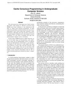
We have developed a new cache profiling tool based on source-level instrumentation. The tool can analyze cache performance of algorithms that operate on STL random access iterators, and we therefore named the tool SMAT (STL Memory Access Tracer). The memory access traces are collected via adaptors, which in STL terminology is a component that wraps another component and provides a modified interface or functionality. The SMAT adaptor provides the same interface as the base component with the additional function of generating traces. SMAT is designed to analyze cache performance of an algorithm, not an entire program. This is often convenient for the study of cache-conscious algorithms. For example, it is common to generate test data and then process it with some algorithm in the same program. In such cases, people usually want to perform cache profiling only for the algorithm code, disregarding the data generation code. Advantages of SMAT over other cache profiling tools can be summarized as follows. • It is portable and independent of hardware architecture since it provides trace functionality at the source level. • It requires little or no modification to the algorithm. However, SMAT expects that the implementation of the algorithm makes all accesses to data sequences through iterators and their associated types. When this is not the case (as may happen if the algorithm is not programmed as generically as it could be), the implementation should be modified to remove the non-iterator accesses. • It is easy to get started with. SMAT only consists of one header file and six utility programs. On the other hand, SMAT has the afore-mentioned drawback of source-based tracers, in that it traces all objects involved whereas the object modification based method only traces real memory accesses and not objects assigned to registers. That is, the source-based trace and object-based trace are collected at different levels of the memory hierarchy, as shown in Figure 1.1. Consequently, SMAT generates much longer traces than the object-based method. Besides, operations of the SMAT-adapted objects cannot be completely optimized by a compiler. The primary theme of this paper is how to deal with these limitations. With a cache simulator that simulates registers as well, and a trace file optimizer that eliminates inefficient memory accesses that would in the absence of tracing be eliminated by the compiler, SMAT provides the convincing cache profiling. The rest of the paper is organized as follows. Section 2 explains how to use SMAT, presenting real example source codes. Section 3 is the reference manual of SMAT adaptor library and utility programs. The design issues are discussed in Section 4. In Section 5, cache performance of STL sorting algorithms is analyzed using SMAT. Improvements of cache-conscious versions of introsort and mergesort over typical implementations are examined as well. Complete source codes of the 6

Target Program Source-based trace is collected here Registers Object-based trace is collected here

Caches

Main Memory

Figure 1.1: Difference between the source-based and object-based trace collection.

SMAT adaptor library, cache simulator, and other utility programs are presented in Appendix A, and Appendix B contains their test suites and results.

7

Chapter 2

User’s Guide 2.1

Overview

SMAT (STL Memory Access Tracer) is a trace-based cache profiling tool to analyze cache performance of algorithms that operate on STL random access iterators. The tool consists of the adaptor library (smat.h), cache simulator (smatsim), trace file optimizer (smatopt), operation counter (smatcount), trace file viewer (smatview), and trace file plotter (smatplot). Figure 2.1 illustrates the flow using SMAT. The caller of the target algorithm is first modified so that the iterator arguments to the target algorithm are wrapped by the SMAT iterator adaptor. Then, the compiled program generates a trace file during its execution. Since the raw trace file may contain inefficient memory references, it is recommended to “optimize” it with the trace file optimizer smatopt. The optimized trace file is processed by the cache simulator smatsim to analyze cache performance. The operation counter smatcount provides the classic operation counting feature, implemented along principles similar to those of OCAL (Operation Counting Adaptor Library) [8], a more general operation counting facility. The trace file plotter smatplot generates a trace plot that exhibits how the algorithm has made memory references over time and which of them incurred cache misses. Such memory access trace plots are an extension of the kind of iterator trace plots produced by the itrace tool [14]. The SMAT adaptor library overloads almost all member functions of the base class and several global functions. Every overloaded function generates a memory access trace implicitly. SMAT can trace memory accesses not only of the iterator type but also of iterator’s associated types. Every STL iterator type has associated types, and SMAT can trace four of them: value type, difference type, pointer type, and reference type. The value type is the type of object to which the iterator points, or the type of *i where i is an iterator. The difference type is a signed integer type that represents the distance between two iterators. The pointer and reference types are simply a pointer and a reference to the value type, respectively. Almost every operation on iterators and associated type objects generates a trace. For example, a statement v = *(i + 1), where i is an iterator and v is a value type object, generates the following trace. (The trace is actually in a binary format and not human-readable. The following output was converted to the human-readable format by the trace file viewer smatview. Comments were added manually.) iaddi readi movv dtori

4, 4, 4, 4,

(0xbffff8b4), (0xbffff884) (0xbffff884) (0xbffff8c8), (0xbffff894) (0xbffff884)

; ; ; ;

8

i + 1 -> tmp *tmp *tmp -> v destruct tmp

target.cpp

smat.h #include

compile

target execute

Trace file

smatopt

Cache performance information

smatsim

smatcount

Operation count information

smatview

Human-readable trace file

smatsim

smatrange

gnuplot

Trace plot

smatplot

Figure 2.1: SMAT flow diagram.

The first trace corresponds to the subexpression i + 1, where i’s address is 0xbffff8b4, and the result is stored into a temporary object at address 0xbffff884. The mnemonic iaddi stands for “immediate addition of the iterator type.” The last letter of the mnemonic, one of i (iterator type), v (value type), d (difference type), p (pointer type), represents the type of object involved. The number 4 after the mnemonic indicates the access length, or the size of the object. The second trace instruction is created by the dereference operation. In that trace, the temporary object is referenced to obtain the address to which the temporary object points. The third trace indicates the assignment, from the address 0xbffff8c8 to v (at address 0xbffff894). The temporary object is no longer necessary and destructed in the last trace instruction.

2.2

Obtaining SMAT

The source archive of SMAT can be found at http://www.cs.rpi.edu/~musser/gp/. See README file in the archive how to configure, compile, and install the SMAT library and utility programs. SMAT has been tested on the following compilers and operating systems. • GCC version 3.2 on Linux 2.4.19, and • GCC version 3.2 on Solaris 5.8. The iterator adaptor (smat.h) requires the Boost Libraries [17], version 1.29.0 or newer. The trace file plotter smatplot requires Gnuplot [9], version 3.7 or newer, and it optionally uses the image compression utility pnmtopng of netpbm [1] to generate PNG format output.

2.3

Example 1 — Reverse a String

In this section, as a first example of how to use SMAT, we measure cache performance of the std::reverse algorithm. Example1a is a small program that reverses a fixed string and prints it 9

out to the standard output. "example1a.cpp" 10a ≡ #include #include #include using namespace std; int main() { string s("Hello, this is SMAT."); reverse(s.begin(), s.end()); cout /dev/null | smatopt | smatcount Iterator: Assignment 21 Comparison 10000 Arithmetic 10000 Value type: Assignment

0

15

Address

(a)

(b)

2000

3000 4000 Clock Cycles

5000

6000

5000

10000 Clock Cycles

15000

20000

Address

0

(c)

1000

Address

0

0

10000

20000 30000 Clock Cycles

40000

50000

Figure 2.3: Trace plots of minmax twopass algorithm, processing (a) 1000, (b) 2500, and (c) 5000 elements.

16

Table 2.1: Comparison of the number of operations.

Number of elements N = 100

N = 1000

N = 10000

N = 100000

Algorithm Two-pass One-pass Fewer cmp. Two-pass One-pass Fewer cmp. Two-pass One-pass Fewer cmp. Two-pass One-pass Fewer cmp.

Comparison Arithmetic

19990 0

Total: Assignment Comparison Arithmetic

21 29990 10000

Assign. 16 12 12 23 18 17 26 21 20 28 23 22

Iterator Comp. Arith. 202 200 100 100 52 202 2002 2000 1000 1000 502 2002 20002 20000 10000 10000 5002 20002 200002 200000 100000 100000 50002 200002

Value type Assign. Comp. Arith. 0 198 0 0 196 0 0 150 0 0 1998 0 0 1993 0 0 1500 0 0 19998 0 0 19990 0 0 15000 0 0 199998 0 0 199989 0 0 150000 0

The number of assignment, comparison, and arithmetic operations are counted separately for each type. The difference type and pointer type are not listed because there were no operations of these types. Section 2.6.5 explains a more detailed report that can be obtained using option -v. Table 2.1 compares the operation counts of three algorithms processing 100–100000 elements. In the fewer-comparisons algorithm, the number of value-type comparisons is 1.5N as intended. The number of iterator type comparisons is fewer than other algorithms as well. The one-pass algorithm performs about a half the iterator comparisons and arithmetic operations of the two-pass algorithm. At N = 100000, the numbers of operations overall are 4000012 in the one-pass algorithm and 400026 in the fewer-comparisons algorithm, showing little difference. However, in terms of clock cycles of the simulator, the one-pass algorithm has 43% fewer cycles than the fewer-comparisons algorithm. This shows that operation counting is not necessarily an appropriate index to compare performance when caches are involved.

2.5

Making the Best Use of SMAT

SMAT expects the algorithm to access memory through operations on iterator types and their associated types. Otherwise, SMAT would miss seeing some memory accesses, which would result in inaccurate cache analysis. For algorithms designed according to generic programming principles as exemplified by STL algorithms, no modification is needed. However, modification to meet the type requirements is sometimes necessary for user-written algorithms. This section gives advice how to modify algorithms so that SMAT can trace all memory accesses.

17

First of all, SMAT is designed to work on STL random access iterators. So the target algorithm must take STL random access iterators as parameters (and possibly others). STL containers that provide random access iterators, in addition to C-style arrays, are std::vector and std::deque1 . SMAT could also be used on algorithms that access a user-defined container if the container provides iterators that meet the STL requirements for random access iterators.

2.5.1

Making Algorithms Analyzeable

Consider the following algorithm, accumulate stride, which accumulates elements of the given vector at positions that are stride apart. Unlike std::accumulate, it does not take an init parameter. The first version is intentionally written in the non-generic style, which is dedicated to container type std::vector. This algorithm will be revised step by step. hAccumulate stride algorithm (not generic). 18ai ≡ int accumulate_stride_1(std::vector& v, int stride) { int sum = 0; for (size_t i = 0 ; i < v.size(); i += stride) sum += v[i]; return sum; } Used in part 115b.

Iterators The first thing that should be done is to parameterize in terms of iterators instead of the container. This is the standard way of the sequence-based generic algorithms of STL. Iterator parameterization provides additional flexibilities. With the following code, for example, a user can now compute the partial stride sum of a sequence instead of an entire sequence. hAccumulate stride algorithm (iterators). 18bi ≡ int accumulate_stride_2(std::vector::iterator first, std::vector::iterator last, int stride) { int sum = 0; for ( ; first < last; first += stride) sum += *first; return sum; } Used in part 115b. 1

Small changes to the iterator adaptor will be required to trace std::deque iterator correctly because the size of std::deque::iterator is larger than that of std::deque::difference type. Section 4.3 describes why this can be a problem.

18

Templates However, just using iterators is not enough because the previous code can only process vector iterators. Making the argument types template parameters provide additional flexibility. In the following code, the iterator type and the type of stride are parameterized. The algorithm can now operate on other types of iterators. hAccumulate stride algorithm (templates). 19ai ≡ template int accumulate_stride_3(T first, T last, U stride) { int sum = 0; for ( ; first < last; first += stride) sum += *first; return sum; } Used in part 115b.

Traits Types Although the parameter types have been templated, the algorithm still assumes that the iterator’s value type is convertible to int, which is not always true. We can obtain the value type — the type of elements to which objects of iterator type T can point — using a library-provided traits class, std::iterator traits::value type. The return type and the type of sum are corrected in the following code. The initialization of sum has changed so that it is now initialized by the first element of the sequence, because initializing by 0 is not generic. Another change is that the addition to sum is done by + instead of += since it makes fewer requirements on the value type. hAccumulate stride algorithm (traits types). 19bi ≡ template typename std::iterator_traits::value_type accumulate_stride_4(T first, T last, U stride) { typename std::iterator_traits::value_type sum(*first); first += stride; for ( ; first < last; first += stride) sum = sum + *first; return sum; } Used in part 115b.

Another Iterator Traits Types So far the algorithm has become fairly generic. It will receive a passing grade in most circumstances. However, SMAT has a stricter requirement. The type of stride is the problem. What will the type of stride be if the function is called as follows? accumulate_stride(v.begin(), v.end(), 5);

The answer is int, which SMAT cannot trace. To trace the third argument, its type must be the iterator’s difference type. 19

hAccumulate stride algorithm (final). 20i ≡ template typename std::iterator_traits::value_type accumulate_stride_final(T first, T last, typename std::iterator_traits::difference_type stride) { typename std::iterator_traits::value_type sum(*first); first += stride; for ( ; first < last; first += stride) sum = sum + *first; return sum; } Used in part 115b.

This technique, specifying the argument type by a traits type, ensures that all arguments are of an iterator type or its associated types.

2.5.2

More Tips

Using Difference Type A user can naturally assume that the difference type is as “powerful” as int type. Therefore, the difference type can be used wherever int type works, and any arithmetic operations applicable to int type can be applied to the difference type. Use the difference type wherever possible and avoid using not-traceable raw types. Making profiling faster In the caller of the algorithm, it is recommended to put the following function calls before the first stream I/O operation. These calls make profiling run much faster (at a factor of 10) on some platforms. std::ios::sync_with_stdio(false); std::cin.tie(0);

2.6 2.6.1

Advanced Topics Disabling SMAT

The memory access tracer can be disabled by replacing all occurrences of smat to Iter manually. However, a much more convenient way is provided, in which a user wraps iterators by smat::type instead of smat. The type smat::type works the same as smat by default. But if the macro SMAT DISABLE is defined, smat::type yields the raw type Iter. The SMAT DISABLE also disables all SMAT macros, such as SMAT SET OSTREAM, by redefining them to do nothing. Therefore, a user can disable SMAT by just defining SMAT DISABLE, without changing the source. But be sure to define SMAT DISABLE before the header file smat.h is included.

20

2.6.2

Viewing Trace Files

The trace file viewer smatview converts a trace file into a human readable format, in which each line of the output corresponds to one trace instruction. A typical trace instruction would look as follows: movv

4, (0x0807e234), (0x0807e20c)

The line consists of the following information. See Section 4.3 for how this information is actually encoded in the raw trace file. • Instruction code — assignment (movv), • Type of object — value type (movv), • Access length — 4, • Source address(es) — 0x0807e234, and • Destination address — 0x0807e20c. The first word, mnemonic, indicates the operation and the type of object. The last letter of the mnemonic, one of i (iterator type), v (value type), d (difference type), p (pointer type), represents the object type. The number that follows the mnemonic is the object size, or the length of the memory access. Hexadecimal numbers enclosed in parentheses are source or destination addresses. Source addresses always precede destination addresses. Every trace instruction takes a fixed number of source or destination addresses. The mov instruction takes one source and one destination address, for example. Sections 3.1–3.5 describe the relationships between SMAT adaptor libraries and trace instructions, and Table 3.1 summarizes them.

2.6.3

Changing Cache Parameters

Cache parameters of the simulator can be changed by recompiling smatsim. A user can modify parameters either by modifying Makefile or specifying them as command line arguments of make. The configurable parameters are as follows. Definitions in Makefile is shown in the parenthesis. The first four parameters must take powers of two, and the write policy must be either true or false. Hit time takes a non-negative integer value. • Number of registers (NREG = 8) • L1 cache capacity (L1 SIZE = 8192) • L1 cache block size (L1 BLOCK = 32) • L1 cache associativity (L1 ASSOC = 2) • L1 cache hit time (L1 LATENCY = 1) • L1 cache write policy (L1 WB = true) • Main memory hit time (MAIN LATENCY = 32) To change the cache size to 16KB, for example, edit Makefile so that the block size parameter is L1 SIZE = 16384, then run make again. $ make smatsim

21

If make command supports defining parameters on the command line, the following would do the same thing. The user does not have to edit Makefile in this case. $ make smatsim L1_SIZE=16384

To avoid confusion, it is recommended give the new simulator a name distinguishable from other versions, for example, smatsim-16kb in this case.

2.6.4

More Cache Performance Information

The cache simulator smatsim outputs more detailed information when -v option is specified. For example, the one-pass algorithm introduced in Section 2.4 generates the following output. $ ./example2 onepass 10000 2>/dev/null | smatopt | smatsim -v Register hits 109994 hits (99977r + 10017w) Register misses 10010 misses (10006r + 4w, 8.34%) Register writebacks 1 (0.00999% of all misses) Register reads 439932 bytes Register writes 40084 bytes L1 L1 L1 L1 L1

cache cache cache cache cache

hits misses writebacks reads writes

8756 hits (8755r + 1w) 1255 misses (1255r + 0w, 12.5%) 1 (0.0797% of all misses) 40040 bytes 4 bytes

Main memory reads Main memory writes

40160 bytes 32 bytes

Total clock cycles

50203 clocks

The output consists of four parts, the information about registers, the level 1 cache, main memory, and clock cycles. The register and L1 cache information look quite similar. In fact, the register set is implemented as the level 0 cache, and so the same statistics are reported for it as for the L1 cache. Having registers in the simulator is essential in SMAT. See Section 4.1.1 for this design decision. Figure 2.4 depicts where these cache statistics are collected in the memory hierarchy. For example, statistics Register reads and Register writes count how many read accesses and write accesses are made by the algorithm, respectively. These accesses cause hits and misses in the register set, and if requests cannot be satisfied within registers, they are forwarded to L1 cache. Statistics L1 cache reads and L1 cache writes count the number of these forwarded accesses. The requests are handled in L1 cache and some of them finally cause main memory accesses. For the number of hits and misses, numbers in the parenthesis indicate how many of them are caused by read requests and write requests, respectively. For example, L1 cache hits

8756 hits (8755r + 1w)

shows that 8755 hits out of 8756 hits are incurred by read requests. The number of misses has an additional number shown as a percentage. L1 cache misses

1255 misses (1255r + 0w, 12.5%)

22

Algorithm Register reads Register writes Register hits Register misses Register writebacks L1 cache hits L1 cache misses L1 cache writebacks

Registers L1 cache reads L1 cache writes

Caches Main memory reads Main memory writes

Main Memory

Figure 2.4: Levels in the memory hierarchy where cache statistics are collected.

The additional number is the miss rate, which is given by the following equation. Number of misses Number of misses = . Number of cache accesses Number of hits + Number of misses So 1255/(8756 + 1255) = 0.125 in the example. A writeback operation occurs in cache block replacement when the block pushed out is dirty. In a cache with write back policy, which is the default policy of smatsim, a writeback operation is the only operation that issues a write request to main memory. A write miss in L1 cache does not issue a write request to main memory. Instead, it issues a read request to bring data to the L1 cache, which is called cache fill. The number of writeback operations is shown in the statistics. The ratio to all the misses is shown as well. L1 cache writebacks

1 (0.0797% of all misses)

Note that writeback operations issue requests to main memory, which take exactly the same number of clock cycles as normal cache misses. So having a large number of writebacks does affect performance. Figure 2.5 summarizes the number of requests issued in each level of the memory hierarchy. All numbers in the statistics and the relationship among them should now be clear. The figure also presents the intuition of how the clock cycles can be computed from the statistics and cache configuration parameters. Total clock cycles = (Number of L1 misses and writebacks) × Hit time Main + (Number of L1 hits and misses) × Hit time L1

(2.1)

In the example, the right-hand side yields (1255 + 1) × 32 + (8756 + 1255) × 1 = 50203, which agrees with the simulated clock cycles. Back to The Fewer-Comparisons Algorithm In Section 2.4.1, the fewer-comparisons algorithm showed poorer performance than expected. Can the detailed cache statistics help explain this result? Here is the output of the fewer-comparisons algorithm, processing the same number of elements as the one-pass algorithm.

23

Algorithm 109994 + 10010 requests (99977 + 10006 reads and 10017 + 4 writes) Registers

Caches

109994 hits, 10010 misses, and 1 writeback. 8756 + 1255 requests (8755 + 1255 reads and 1 write) 8756 hits, 1255 misses, and 1 writeback. 1255 + 1 requests (1255 reads and 1 write)

Main Memory

Figure 2.5: Number of requests issued at each level in the memory hierarchy.

$ ./example2 fewercmp 10000 2>/dev/null | smatopt | smatsim -v Register hits 62337 hits (57321r + 5016w) Register misses 47713 misses (32707r + 15006w, 43.4%) Register writebacks 20 (0.0419% of all misses) Register reads 360112 bytes Register writes 80088 bytes L1 L1 L1 L1 L1

cache cache cache cache cache

hits misses writebacks reads writes

46452 hits (46432r + 20w) 1281 misses (1281r + 0w, 2.68%) 1 (0.0781% of all misses) 190852 bytes 80 bytes

Main memory reads Main memory writes

40992 bytes 32 bytes

Total clock cycles

88757 clocks

Compared to the output from one-pass algorithm, the fewer-comparisons algorithm clearly makes many register misses (10010 v.s. 47713), while total number of register reads and writes is comparable (439932 + 40084 = 480016 v.s. 360112 + 80088 = 440200, in bytes). This implies that the fewer-comparisons algorithm has less locality in memory references. Recalling that the fewer-comparisons algorithm made a large number of misses in iterator accesses, we conclude that the fewer-comparisons algorithm shows poorer performance because the iterator accesses have less locality. See Section 4.2.2 for how this can be improved.

2.6.5

Detailed Operation Counting

The operation counter smatcount provides more detailed information with the -v option. In the detailed format, operation counts are decomposed into the operator function level. For example, the one-pass algorithm processing 10000 elements generates the following. $ ./example2 onepass 10000 2>/dev/null | smatopt | smatcount -v Iterator: Ctor (copy) 2 Ctor (base type) 2

24

Dtor = != ++

4 17 10000 10000

Value type:
rhs.base(). SMAT GT. template bool operator= rhs.base(). SMAT GEQ.

3.2

Difference Type Adaptor

3.2.1

Files

#include "smat.h"

3.2.2

Class Declaration

template class smat_d

29

3.2.3

Description

The difference type adaptor class smat d wraps the base difference type T, which is given as the template parameter, and emulates T. At the same time, it generates a memory access trace of almost all operations by overloading them. The trace codes assigned to overloaded functions are shown at the end of each function description. Since the base type T is usually defined as int or long int, smat d overloads all possible operations that can be applied to these integral types.

3.2.4

Constructors, Destructors, and Related Functions

smat_d();

Default constructor. SMAT CTOR. smat_d(const smat_d& x);

Copy constructor. SMAT CCTOR. smat_d(const T& x);

Constructs a smat d object from the base difference type object x. SMAT BCTOR. operator T() const;

Conversion operator to the base difference type. SMAT READ. smat_d& operator=(const smat_d& x)

Assignment operator. SMAT MOV. ~smat_d();

Destructor. SMAT DTOR.

3.2.5

Public Member Functions

const T& base() const;

Returns the const reference to the base difference type object. smat_d& operator++(); smat_d operator++(int);

Prefix and postfix increment operator. SMAT INC. smat_d& operator--(); smat_d operator--(int);

Prefix and postfix decrement operator. SMAT DEC. smat_d& operator+=(const smat_d& x);

30

Calls base() += x.base() and returns *this. SMAT ADD. smat_d& operator-=(const smat_d& x);

Calls base() -= x.base() and returns *this. SMAT SUB. smat_d& operator*=(const smat_d& x);

Calls base() *= x.base() and returns *this. SMAT MUL. smat_d& operator/=(const smat_d& x);

Calls base() /= x.base() and returns *this. SMAT DIV. smat_d& operator%=(const smat_d& x);

Calls base() %= x.base() and returns *this. SMAT MOD. smat_d& operator= x.base() and returns *this. SMAT RSHIFT. smat_d& operator&=(const smat_d& x);

Calls base() &= x.base() and returns *this. SMAT AND. smat_d& operator|=(const smat_d& x);

Calls base() |= x.base() and returns *this. SMAT OR. smat_d& operator^=(const smat_d& x);

Calls base() ^= x.base() and returns *this. SMAT XOR. template smat_d& operator+=(const U& x);

Calls base() += x and returns *this. SMAT IADD. template smat_d& operator-=(const U& x);

Calls base() -= x and returns *this. SMAT ISUB. template smat_d& operator*=(const U& x);

Calls base() *= x and returns *this. SMAT IMUL. template smat_d& operator/=(const U& x);

Calls base() /= x and returns *this. SMAT IDIV. 31

template smat_d& operator%=(const U& x);

Calls base() %= x and returns *this. SMAT IMOD. template smat_d& operator= x and returns *this. SMAT IRSHIFT. template smat_d& operator&=(const U& x);

Calls base() &= x and returns *this. SMAT IAND. template smat_d& operator|=(const U& x);

Calls base() |= x and returns *this. SMAT IOR. template smat_d& operator^=(const U& x);

Calls base() ^= x and returns *this. SMAT IXOR. smat_d* operator&(); const smat_d* operator&() const;

Address-of operator. This operator does not have a trace instruction code because no memory reference is involved in returning a pointer. smat_d operator+() const;

Returns smat d(base()). The assigned trace instruction code is SMAT READ, since it is not that interesting to trace the unary plus operator. smat_d operator-() const;

Returns smat d(-base()). SMAT MINUS. smat_d operator~() const;

Returns smat d(~base()). SMAT CMPL.

3.2.6

Global Operations

template const smat_d operator+(const smat_d& lhs, const smat_d& rhs);

Addition operator between two smat d objects. Returns lhs.base() + rhs.base(). SMAT ADD.

32

template const smat_d operator+(const smat_d& lhs, const U& rhs); template const smat_d operator+(const U& lhs, const smat_d& rhs);

Addition operators between smat d and an integral constant. Return lhs.base() + rhs and lhs + rhs.base(), respectively. SMAT IADD. template const smat_d operator-(const smat_d& lhs, const smat_d& rhs);

Returns lhs.base() - rhs.base(). SMAT SUB. template const smat_d operator-(const smat_d& lhs, const U& rhs); template const smat_d operator-(const U& lhs, const smat_d& rhs);

Return lhs.base() - rhs and lhs - rhs.base(), respectively. SMAT ISUB. template const smat_d operator*(const smat_d& lhs, const smat_d& rhs);

Returns lhs.base() * rhs.base(). SMAT MUL. template const smat_d operator*(const smat_d& lhs, const U& rhs); template const smat_d operator*(const U& lhs, const smat_d& rhs);

Return lhs.base() * rhs and lhs * rhs.base(), respectively. SMAT IMUL. template const smat_d operator/(const smat_d& lhs, const smat_d& rhs);

Returns lhs.base() / rhs.base(). SMAT DIV. template const smat_d operator/(const smat_d& lhs, const U& rhs); template const smat_d operator/(const U& lhs, const smat_d& rhs);

Return lhs.base() / rhs and lhs / rhs.base(), respectively. SMAT IDIV. template const smat_d operator%(const smat_d& lhs, const smat_d& rhs);

Returns lhs.base() % rhs.base(). SMAT MOD. template const smat_d operator%(const smat_d& lhs, const U& rhs); template const smat_d operator%(const U& lhs, const smat_d& rhs);

33

Return lhs.base() % rhs and lhs % rhs.base(), respectively. SMAT IMOD. template const smat_d operator> rhs and lhs >> rhs.base(), respectively. SMAT IRSHIFT. template const smat_d operator&(const smat_d& lhs, const smat_d& rhs);

Returns lhs.base() & rhs.base(). SMAT AND. template const smat_d operator&(const smat_d& lhs, const U& rhs); template const smat_d operator&(const U& lhs, const smat_d& rhs);

Return lhs.base() & rhs and lhs & rhs.base(), respectively. SMAT IAND. template const smat_d operator|(const smat_d& lhs, const smat_d& rhs);

Returns lhs.base() | rhs.base(). SMAT OR. template const smat_d operator|(const smat_d& lhs, const U& rhs); template const smat_d operator|(const U& lhs, const smat_d& rhs);

Return lhs.base() | rhs and lhs | rhs.base(), respectively. SMAT IOR. template const smat_d operator^(const smat_d& lhs, const smat_d& rhs);

Returns lhs.base() ^ rhs.base(). SMAT XOR. template const smat_d operator^(const smat_d& lhs, const U& rhs); template const smat_d operator^(const U& lhs, const smat_d& rhs);

Return lhs.base() ^ rhs and lhs ^ rhs.base(), respectively. SMAT IXOR. 34

3.2.7

Equality and Ordering Predicates

template bool operator==(const smat_d& lhs, const smat_d& rhs);

Returns lhs.base() == rhs.base(). SMAT EQ. template bool operator!=(const smat_d& lhs, const smat_d& rhs);

Returns lhs.base() != rhs.base(). SMAT NEQ. template bool operator(const smat_d& lhs, const smat_d& rhs);

Returns lhs.base() > rhs.base(). SMAT GT. template bool operator= rhs.base(). SMAT GEQ. template bool operator==(const smat_d& lhs, const U& rhs); template bool operator==(const U& lhs, const smat_d& rhs);

Equality test between integral constants. Returns lhs.base() == rhs and lhs == rhs.base(), respectively. SMAT IEQ. template bool operator!=(const smat_d& lhs, const U& rhs); template bool operator!=(const U& lhs, const smat_d& rhs);

Returns lhs.base() != rhs and lhs != rhs.base(), respectively. SMAT INEQ. template bool operator(const U& lhs, const smat_d& rhs);

Returns lhs.base() > rhs and lhs > rhs.base(), respectively. SMAT IGT. template bool operator= rhs.base(), respectively. SMAT IGEQ. 35

3.3

Value Type Adaptor

3.3.1

Files

#include "smat.h"

3.3.2

Class Declaration

template class smat_v

3.3.3

Description

The value type adaptor class smat v wraps the base value type T, and emulates T. At the same time, it generates a memory access trace of almost all operations by overloading them. Further description is omitted because the interface of smat v is exactly the same as the difference type adaptor smat d, except that smat d has the addition operators with iterator types and that the subtraction between iterators yields type smat d.

3.4

Pointer Type Adaptor

3.4.1

Files

#include "smat.h"

3.4.2

Class Declaration

template class smat_p

3.4.3

Description

The pointer type adaptor class smat p wraps the base pointer type T and emulates T. At the same time, it generates a memory access trace of almost all operations by overloading them. Most of the descriptions of functions of this class are omitted because they are identical to those of smat. Only functions that are not defined in smat are described below.

3.4.4

Public Member Functions

smat_p& operator=(smat_v* x)

Assignment operator from the pointer of the value type object. SMAT MOV.

3.5

Trace Instruction Code

3.5.1

Files

#include "smat.h"

3.5.2

Class Declaration

enum smat_code

36

3.5.3

Description

The smat code enumeration defines constants that identify each trace instruction. Although this enumeration is only used internally, the correspondence between the trace instruction codes and SMAT adaptor library functions is important to understanding how SMAT works. Briefly, every SMAT adaptor library function described in preceding sections has a corresponding trace instruction code and generates the trace of the assigned code at every invocation. Some instructions have their “immediate version” counterparts. For example, SMAT IADD is the immediate version of SMAT ADD. The immediate version is generated by the expression in which one of the operands is an immediate value, or a constant. For example, an expression i + 1, where i is an iterator, generates the instruction code SMAT IADD.

3.5.4

Enumerator Constants

SMAT_CCTOR

Generated by copy constructors. SMAT_BCTOR

Generated by conversion operators from the base type objects. SMAT_CTOR

Generated by default constructors. This instruction is not printed by smatview. (Use option -v to print). SMAT_DTOR

Generated by destructors. SMAT_MOV

Generated by assignment operators. SMAT_AND SMAT_IAND

Generated by bitwise and operators. SMAT IAND is generated when one of the operands is an immediate value. SMAT_OR SMAT_IOR

Generated by bitwise or operators. SMAT_XOR SMAT_IXOR

Generated by bitwise xor operators. SMAT_INC

37

Generated by both prefix and postfix increment operators. SMAT_DEC

Generated by both prefix and postfix decrement operators. SMAT_CMPL

Generated by complement operators. SMAT_MINUS

Generated by unary minus operators. SMAT_ADD SMAT_IADD

Generated by addition operators. SMAT_SUB SMAT_ISUB

Generated by subtraction operators. SMAT_MUL SMAT_IMUL

Generated by multiplication operators. SMAT_DIV SMAT_IDIV

Generated by division operators. SMAT_MOD SMAT_IMOD

Generated by modulo operators. SMAT_LSHIFT SMAT_ILSHIFT

Generated by left shift operators. SMAT_RSHIFT SMAT_IRSHIFT

Generated by right shift operators. SMAT_EQ SMAT_IEQ

Generated by equality operators. 38

SMAT_NEQ SMAT_INEQ

Generated by inequality operators. SMAT_GT SMAT_IGT

Generated by greater-than operators. SMAT_GEQ SMAT_IGEQ

Generated by greater-than-or-equal-to operators. SMAT_LT SMAT_ILT

Generated by less-than operators. SMAT_LEQ SMAT_ILEQ

Generated by less-than-or-equal-to operators. SMAT_NOP

Generated when the trace file optimizer has eliminated an instruction. This instruction is not printed by smatview. (Use option -v to print.) SMAT_READ

Indicates arbitrary memory read. Generated by dereference, subscripting, arrow, unary plus operators, and conversion operators to the base types. SMAT_WRITE

Indicates arbitrary memory write. Currently not used. SMAT_FMARK

Places some mark in trace files. Currently not used.

3.5.5

Trace Instruction Summary

Table 3.1 is the complete list of trace instructions. The table consists of the instruction code, mnemonic (used in smatview), the number of source addresses and destination addresses, corresponding operator function, and notes.

39

Table 3.1: Trace instruction summary. Code Mnemonic Src.† Dest.‡ SMAT CCTOR cctor 1 1 SMAT BCTOR bctor 1 1 SMAT CTOR ctor 0 0 SMAT DTOR dtor 1 0 SMAT MOV mov 1 1 SMAT AND and 2 1 SMAT OR or 2 1 SMAT XOR xor 2 1 SMAT IAND iand 1 1 SMAT IOR ior 1 1 SMAT IXOR ixor 1 1 SMAT INC inc 1 1 SMAT DEC dec 1 1 SMAT CMPL cmpl 1 1 SMAT MINUS minus 1 1 SMAT ADD add 2 1 SMAT SUB sub 2 1 SMAT MUL mul 2 1 SMAT DIV div 2 1 SMAT MOD mod 2 1 SMAT LSHIFT sl 2 1 SMAT RSHIFT sr 2 1 SMAT IADD iadd 1 1 SMAT ISUB isub 1 1 SMAT IMUL imul 1 1 SMAT IDIV idiv 1 1 SMAT IMOD imod 1 1 SMAT ILSHIFT isl 1 1 SMAT IRSHIFT isr 1 1 SMAT EQ eq 2 0 SMAT NEQ neq 2 0 SMAT GT gt 2 0 SMAT GEQ geq 2 0 SMAT LT lt 2 0 SMAT LEQ leq 2 0 SMAT IEQ ieq 1 0 SMAT INEQ ineq 1 0 SMAT IGT igt 1 0 SMAT IGEQ igeq 1 0 SMAT ILT ilt 1 0 SMAT ILEQ ileq 1 0 SMAT NOP nop 0 0 SMAT READ read 1 0 SMAT WRITE write 0 1 SMAT FMARK mark 0 0 † The number of source addresses. ‡ The number of destination addresses.

Operator

= & | ^ & | ^ ++ -~ - (unary) + * / % > + * / % > == != > >= < >= <

40

Notes copy constructor conversion from the base type default constructor destructor assignment bitwise and bitwise or bitwise xor bitwise and with immediate value bitwise or with immediate value bitwise xor with immediate value increment (both pre and post) decrement (both pre and post) unary bitwise complement unary minus addition subtraction multiplication division modulo left shift right shift addition with immediate value subtraction with immediate value multiplication with immediate value division with immediate value modulo with immediate value left shift with immediate value right shift with immediate value equality inequality greater than greater than or equal to less than less than or equal to comparison with immediate value likewise likewise likewise likewise likewise do nothing read operation not used not used

3.5.6

Expression Examples and Corresponding Traces

For a number of statements and expressions, their corresponding traces are presented. “Pseudo” trace instructions are used in which the address of object i is shown as (i) instead of its raw address. Additionally the following assumptions are made. • Iter denotes the SMAT-adapted iterator type. • i and j denote variables of type Iter. • d and n denote variables of Iter’s difference type. • v denotes a variable of Iter’s value type. Iter i(j); cctori

4, (j), (i)

; copy j to i

4, (i), (tmp) 4, (tmp), (j) 4, (tmp)

; i + 1 -> tmp ; tmp -> j ; destruct tmp

4, (i), (tmp) 4, (j), (tmp) 4, (tmp)

; i + 100 -> tmp ; j >= tmp ; destruct tmp

4, (j), (i), (tmp) 4, (tmp), (d) 4, (tmp)

; j - i -> tmp ; tmp -> d ; destruct tmp

4, (d), (tmp) 4, (tmp), (n) 4, (tmp)

; d * 2 -> tmp ; tmp -> n ; destruct tmp

4, (d), (d)

; d * 2 -> d

4, (i) 4, (*i), (v)

; read from i ; copy *i to v

4, 4, 4, 4,

; ; ; ;

j = i + 1; iaddi movi dtori j >= i + 100 iaddi gteqi dtori d = j - i; subi movd dtord n = d * 2; imuld movd dtord d *= 2; imuld v = *i; readi movv v = *(i + 1); iaddi readi movv dtori

(i), (tmp) (tmp) (*tmp), (v) (tmp)

i + 1 -> tmp read from tmp copy *tmp to v destruct tmp

41

3.6

Cache Simulator

3.6.1

Synopsis

smatsim [OPTION]... < TRACEFILE

3.6.2

Description

The cache simulator for SMAT. It reads a trace file from the standard input, performs the cache simulation, and then outputs the cache statistics to the standard output stream. Cache parameters are given at compile-time. See Section 2.6.3 for how to change cache parameters.

3.6.3

Options

-c

Display cache parameters and exit. -d

Generate debug outputs. With -d option, it prints every trace instruction simulated, as well as the current clock count. With -dd option, it also dumps all non-empty cache block information after each step, in a format like *bffff780-9f:60:238. The first asterisk indicates the block is dirty. The next hexadecimal numbers are the address range to which the block corresponds. The next decimal number (60) is the set index. The last number (238) is the time in clock cycles when the block is last used. Some entries might have

iaddi nop nop

4, (i), (j)

In the original instructions (left-hand side), the result of i + 1 is once written to the temporary object, and then copied to j, followed by a destruction of the temporary object. References to the temporary object are useless and so the instructions can be optimized as in the right-hand side, in which the result of i + 1 is directly written to j and the references to the temporary object are eliminated. Early Destruction “Early destruction” is the optimization that destructs objects as early as possible. Specifically, it moves destructors just after the trace instruction in which the destructed object is last used. Since the destructor may “free” a register in the simulation, this optimization can improve register utilization. The following is the example of early destruction. In the left-hand side, it is assumed that x is no longer used after the first imuld instruction and y is last used in ineqd instruction. Then, in the right-hand side, destructors of x and y are moved just after the instruction in which they are last used.

51

imuld : : ineqd : : dtord dtord

4, (x), (y)

4, (y)

->

4, (y) 4, (x)

imuld dtord : ineqd dtord : nop nop

4, (x), (y) 4, (x) 4, (y) 4, (y)

Copy Propagation If an object y is written once by the assignment-like trace instruction (SMAT MOV, SMAT CCTOR, and SMAT BCTOR) and just referred to many times thereafter, read accesses to y can possibly be eliminated by copy propagation. The following pseudo instructions illustrates the idea. cctord : subd : eqd : dtord

4, (x), (y) 4, (y), ... -> 4, (y), ... 4, (y)

nop : subd : eqd : nop

4, (x), ... 4, (x), ...

In the left-hand side, an object y is copied from object x, and is read many times by other instructions. This sequence can be optimized as in the right-hand side. The read references to y are replaced by references to x. The instructions to create and destroy y are eliminated as well.

4.2.2

Weakness — Lack of Common Subexpression Removal

The trace optimizer, however, does not necessarily eliminate all ineffective memory accesses. One of its significant weaknesses is that it cannot eliminate common subexpressions. Common subexpression elimination (CSE) is an important compile-time optimization in which each common subexpression is computed only once, then the result is referred to from other contexts. However, CSE does not work for expressions of SMAT-adapted objects since eliminating them has side effects. Unfortunately, the trace file optimizer smatopt cannot perform CSE neither. Users are therefore advised to avoid writing algorithm code in which the same subexpression appears many times, by referring instead to a temporary variable introduced to hold the value of the expression. The algorithm minmax fewercmp introduced in Section 2.4 is an example for which manual CSE is effective. In minmax fewercmp, the subexpression first + 1 is computed twice per loop (once in the if statement and once as the parameter of minmax helper), and first + 2 is computed every time in the conditional expression of the for statement. The following is a modified version of minmax fewercmp. The subexpression first + 1 is eliminated by introducing a new variable first plus one. The conditional expression in the for loop first + 2