Genetic Algorithm-based Robot Path Planning Mohd Faisal Ibrahim, Adilah Zaira Abu Bakar and Aini Hussain Department of Electrical, Electronics and Systems Engineering, Faculty of Engineering and Built Environment, Universiti Kebangsaan Malaysia, 43600 UKM Bangi, Selangor, MALAYSIA Email:
[email protected]
Abstract Nowadays, building an intelligent robot that able to move by itself from one location to another without collides with other obstacles is of interest in many applications. In the real world, condition of an environment is always unpredictable and changes with the existence of dynamic obstacles. This paper tends to propose an algorithm for robot path planning in a dynamic environment using Genetic algorithm (GA) technique. The proposed algorithm is able to find an optimum path for a robot and avoid any static and dynamic obstacles. The variation of the proposed algorithm is shown with the implementation of the algorithm in 4-way movement robot and 8-way movement robot. The simulation results show significant performance of the algorithm when compared with real optimum path.
1. Introduction Path planning mechanism has been applied into many latest applications that required automatic path control such as UAV (Unmanned Vehicle Aerial), UGV (Unmanned Ground Vehicle), rescue robots, rocket and missile. This intelligent-like mechanism basically has the typical aim to move an object from one position to another determined position via the possible shortest path without collides with any obstacles. In this paper, a Genetic algorithm (GA)-based path planning algorithm is introduced for small-scaled robot movement in dynamic environment. The algorithm considers method of handling static obstacles and dynamic obstacles. One of the important elements of the robot path planning is the ability to response to the changes of environment. Initially, the robot path is pre-determined based on static obstacles occurred in any possible path. However, when robot moves after certain moment, surrounding environment may change due to existence
of dynamic obstacles in the pre-determined path. The mechanism should be able to immediately identify new path before robot collides with dynamic obstacles that suddenly obstruct the current path. This paper is organized as follow: the next section will discuss on parameters used for determining robot’s path. Then, implementations of GA in path planning and program development are presented. The simulation result and comparison between two different parameters used are discussed and finally followed by future work and conclusion. 2. Robot Path Parameters Selection of path parameters is the first task that should be taken in path planning. Examples of path parameter are movement angle, movement distance, movement direction etc. These parameters become the guidance for action of a robot. In [3], 3D movement is used as path parameter. Although the final result of the work has shown good performance but there are many mathematical equations used which are time consuming and impractical for real-time application. In this paper, two types of path parameter are chosen because of its simplicity in calculation but maintains reliable. The first parameter is 4-way movement and the second parameter is 8-way movement. As in figure 1(a), the 4-way movement is a combination of four determined direction which is north (0), south (2), west (3) and east (1). Meanwhile, the 8way movement is an addition of 4-way movement with another 4 directions as in figure 1(b).
(a)
(b)
Figure 1. (a) 4-way movement (b) 8-way movement
Optimum path can be measured by using distance and time taken to move a robot from an initial location to a final location. Distance can be calculated by using simple mathematical equation or Pythagoras’s theorem. Time taken can be reduced by finding path with the smallest changes of direction of movement. In this case, both distance and time will be used as measurement parameters to automatically find the possible optimum path of a robot. GA will use both parameters to identify optimum path as will be described in details in the following section. 3. Identification of optimum path using GA Many algorithms have been proposed to develop effective mechanism for automatic robot path planning [1][3][5]. However, GA has shown significance performance compared to other algorithms in term of reliability. GA is a class of stochastic search algorithms based on biological evolution [4]. It does not require derivative information; it can provide a list of optimum parameters, not just a single solution [2]. Considering these facts, robot path optimization can be performed effectively with GA because the algorithm performs a parallel, but directed search to evolve the most fitted solution in a systematic approach. 3.1. Chromosome representation Each gene in a chromosome is encoded with suitable parameter to allow GA to search the best path solution. Direct encoding is used to ensure simplicity and reliability in term of fast processing approach. In this paper, each chromosome of GA represents a collection of next direction of movement in every location point starting from initial point to end point as shown in figure 2 below:Dinitial_point
Dnext_point
Dnext_point
…… Dfinal_point-1
where, D = integer represents direction to next point. Figure 2. Chromosome representation Information in each gene can be used to identify the next coordinate or location that a robot should move. Number of genes in a chromosome is determined based on the minimum steps taken to reach the final point. 3.2. Cost function Before ‘selection’, ‘crossover’ and ‘mutation’ processes can be executed in GA, cost function which determines the target of GA search must be decided. As
stated before, path distance and time taken to move a robot from an initial location to a final location can be used as the cost function in GA. Equation 1 below is used to calculate the cost function:(1) where, w1, w2, w3: constants D: differential distance O: a number of path coordinates matches with obstacles coordinates. C: a number of changes of direction Chromosome with the lowest cost function is said to have the best solution. Differential distance will be used to identify the difference between final location produced by each chromosome and the desired final location. Each chromosome will be read to get the final coordinate of each possible path. If the final coordinate matches the desired destination of robot, the differential distance value will be zero which in turn will produce lower cost function value. On the other hand, time taken can be reduced by counting number of changes of direction in the whole path. It is assumed that, time will increase proportional with the number of changes of direction. This cost function also has direct relation to identify whether a suggested path collides with obstacles or not. Each location point in a suggested path will be checked with obstacle position. The cost function will increase drastically if any of the point matches obstacle position. Therefore, the best solution is said to have the lowest differential distance, the lowest number of changes of direction and the lowest number of collision with obstacles. Figure 3 shows how the cost function is used to converge possible paths to the best solution. Once the encoding of the chromosomes and the cost function had been determined, the algorithm of an automatic robot path planning can be developed as follows: 1. Define string with necessary length to represent parameter of whole path. 2. Make random initial population. 3. Evaluate individual fitness for every chromosome using cost function. 4. Perform selection, crossover and mutation operation with binary string representation to produce new population. 5. Repeat step 3 and 4 until certain generation (set by user) to get the best chromosome. 6. Using the best chromosome, the best path in term of distance and time to reach destination will be obtained.
4.1 Path planning with static obstacles consideration Cost function plays an important part in obtaining the optimum path that can avoid robot from collides with static obstacles. For the cost function calculation, it will start with initial coordinate at 0,0 assuming as the starting position of robot. Whenever a gene value (represents next direction of movement) is obtained, current coordinate will be changed according to respective gene’s direction. The updated coordinate will then be compared with static obstacles’ coordinate. If the coordinate matches with any static obstacles’ position, the cost function for the path formed by particular chromosome will be doubled to a large number to reduce the probability of the chromosome to be selected for next generation. By using this strategy, ‘unfitted’ chromosome can be eliminated very quickly and make convergence process faster.
start
Set initial coordinate = 0,0
i=
Read gene[i] of a chromosome
Update coordinate based on gene[i] value
New coordinate = obstacle coordinates?
Yes Add O with 1
No gene[i] = gene[i+1] ? No
Yes Add C with 1
i+ Yes
i < total genes? No
Calculate cost function using equation 1
stop Figure 3. Cost function usage 4. Program development for robot path planning In general, the robot path planning program holds two main components. Both components involve GA execution to find optimum path with determined parameters. The first component caters path planning with static obstacles consideration which is always executed prior to robot movement. The second component involves path re-planning with dynamic obstacles consideration. The second component is only performed when robot has moved and there is obstacle suddenly appears on the pre-determined path. In this paper, LabView software has been used to develop the program. The following sub-sections will further discuss both of the components of the program.
4.2 Path planning with dynamic obstacles consideration In the real world, dynamic obstacles can only be detected when robot moves approaching that obstacle using specific sensor. As such, the developed program can only detect dynamic obstacles when simulation of robot movement is executed. At any time during simulation, when dynamic obstacle appears, the robot stops, some parameters are changed and the second component of the program will be immediately executed to find new path. The changed parameters include number of gene for each chromosome, initial coordinate based on the latest robot coordinate and new obstacles’ coordinate matrix. When the new path is acquired, the robot will move again until another dynamic obstacle turns up. The process repeats until the robot reaches the final position. 5. Simulation result and comparison Few simulations were conducted to analyze the effectiveness of GA technique as the path planning algorithm. Both 4-way movement and 8-way movement approaches were simulated and presented. At the end, the result from both approaches is compared. 5.1. Simulation in environment with static obstacles For the first experiment, only static obstacles were added into simulated environment. The initial coordinate is set to 0,0 meanwhile the final coordinate is randomly set. Here, coordinate 15,9 is selected which means the final coordinate has distance 15 units to east and 9 units to south from the initial coordinate. Figure 4 shows the simulation results using 4-way movement and 8-way movement robots. The first simulation was done with random cluttered obstacles (figure 4a and 4b). Then, the second simulation was executed with regional
obstacles (figure 4c and 4d) and the final simulation was performed with obstacles surrounds the final coordinate (figure 4e and 4f). From figure 4, it has shown in general the capability of GA to find the optimum path regardless of any formation of static obstacles. In comparison, 8-way movement robot gives better path from 4-way movement robot with smaller changes of direction. Simulation 1- Cluttered obstacles Initial point
Final point
executed before simulating the robot movement. Later, during the simulation, two dynamic obstacles were added in two different periods and the second component of the program as elaborated in section 4 is executed. Figure 5 illustrates the simulation results using 4-way movement and 8-way movement robots. In figure 5(a) and 5(b), the original paths were defined using the first component. When a dynamic obstacle was added, the paths have changed as in figure 5(c) and 5(d) accordingly. Again, when the second dynamic obstacle was detected, the second component was executed to find the latest paths that should be taken by the robots (figure 5e and 5f). Based on these results, it has shown that the proposed algorithm was able to find the best path and avoid any obstacles exist on the path way. Simulation 4 - Original path
4-way movement
8-way movement
(a)
(b)
Simulation 2 – Regional obstacles
4-way movement
8-way movement
(a)
(b)
Simulation 5 - Updated path (dynamic obstacle #1 detected) 4-way movement
8-way movement
(c)
(d)
Simulation 3 – Obstacles surround final point
4-way movement
8-way movement
(c)
(d)
Simulation 6 - Updated path (dynamic obstacle #2 detected) 4-way movement
8-way movement
(e)
(f)
Static obstacle
Path
Figure 4. Simulation results in environment with static obstacles 4-way movement
5.2. Simulation in environment with static and dynamic obstacles In order to investigate the efficiency of the whole program, static and dynamic obstacles were added up into the environment. Static obstacles were defined randomly and the first component of the program was
8-way movement
(e) Static obstacle
(f) Dynamic obstacle
Figure 5. Simulation results in environment with static and dynamic obstacles
5.3 Analysis on algorithm efficiency level The experiments in section 5.1 and 5.2 have shown the capability of the GA-based path planning algorithm to determine the optimum path for a robot to reach final position. Another experiment was also conducted to compare the path produced by the algorithm with the real optimum path identified manually. Figure 6 shows various paths comparison. According to figure 6(a), 6(b) and 6(f), the path generated by the GA-based path planning algorithm is completely matched with the real optimum path. For simulation 8 and 9 in figure 6(c), 6(d) and 6(e), the results from the algorithm are slightly different but nearly approaching the real optimum paths which can be considered as accepted variation. Table 1 indicates the differences between the generated paths from the algorithm and the real optimum paths. Simulation 7 - Environment with no obstacle
4-way movement
(a)
8-way movement
(b)
Simulation 8 - Environment with cluttered obstacles
4-way movement
(c)
8-way movement
(d)
Table 1. Differences between the generated paths from GA-based path planning algorithm and the real optimum paths Simulation #
No. of changes of direction Real
#7 (4-way) Figure. 6(a) #7 (8-way) Figure. 6(b) #8 (4-way) Figure 6(c) #8 (8-way) Figure 6(d) #9 (4-way) Figure 6(e) #9 (8-way) Figure 6(f)
No. of unit distance taken to reach final point GA-based Real GA-based
1
1
24
24
1
1
15
15
4
6
24
24
2
4
15
15
1
3
24
24
1
1
15
15
Another comparison that can be made is the results produced by 4-way movement and 8-way movement approaches. From Table 2, it can be seen that 8-way movement approach generates shorter path distance compared to 4-way movement approach. Number of changes of direction is also smaller in 8-way movement approach which reduces time taken for robot to reach final location. Therefore, it can be concluded that 8-way movement approach is better than 4-way movement approach. 6. Future work To further improve the algorithm proposed in this paper, some improvements are planned. The focus of the improvements includes the study to develop hybrid algorithm of GA with other technique and also determine better approach to find appropriate number of genes in a chromosome so that level of efficiency can be further increased.
Simulation 9 - Environment with regional obstacles
7. Conclusion In conclusion, the path planning algorithm has been successfully developed using GA technique. It is proven based on the discussed result, the optimum paths produced by the algorithm can move a robot from initial location to final location without collide with static or dynamic obstacles. 4-way movement
(e)
8-way movement
(f)
Figure 6. Various paths comparison
References [1] Diosi A. et.al., "Interactive SLAM using Laser and Advanced Sonar", Proc. International Conference on Robotic and Automation, pp. 1103-1108, 2005. [2]Haupt R.L & Haupt S.E., Practical Genetic Algorithms, John Wiley & Sons, 1998. [3] Masehian E. & Habibi G., “Robot Path Planning in 3D Space Using Binary Integer Programming”, International Journal of Mechanical Systems Science and Engineering, Vol.1, No. 1, pp. 26-31, 2007. [4] Negnevitsky M., Artificial Intelligence: A Guide to Intelligent Systems, Addision-Wesley, 2005. [5] Stentz A., “Optimal and Efficient Path Planning for Partially-Known Environments”, Proc. International Conference on Robotic and Automation, pp. 3310-3317, 1994.