In this paper we present a simplified model of parallel, on-chip buses, motivated by the movement toward CMOS technologies where the ratio between inter-wire ...
A Power-Efficient, Low-Complexity, Memoryless Coding Scheme for Buses with Dominating Inter-Wire Capacitances Tina Lindkvist, Jacob Löfvenberg, Henrik Ohlsson, Kenny Johansson and Lars Wanhammar Department of Electrical Engineering, Linköpings Universitet, SE-581 83 Sweden {tina, jacob, henriko, kennyj, larsw}@isy.liu.se
Abstract In this paper we present a simplified model of parallel, on-chip buses, motivated by the movement toward CMOS technologies where the ratio between inter-wire capacitance and wire-to-ground capacitance is very large. We also introduce a ternary bus state representation, suitable for the bus model. Using this representation we propose a coding scheme without memory which reduces energy dissipation in the bus model by approximately 2030% compared to an uncoded system. At the same time the proposed coding scheme is easy to realize, in terms of standard cells needed, compared to several previously proposed solutions.
1. Introduction 1.1. Background The continuing decrease in the minimum feature size in modern CMOS circuits and the corresponding increase in chip density and operating frequency have made power consumption a major concern in ULSI design. Chip area and throughput may no longer be primary system limiting factors except in very high-volume integrated circuits (tens of millions circuits per year) and in general-purpose computing. What is becoming a more and more important factor in CMOS circuits is consumption and dissipation of power. One of the reasons for this is the increase in the number of hand-held devices, requiring electronic circuits with low power consumption to increase battery time. In this paper our concern is not high-speed, but instead very low power. This means that the buses we consider are energy optimized, even if this means that we have to sacrifice throughput. As a result, problems with cross-talk and inductive couplings will not be discussed. One important factor in power consumption, and one that needs addressing, is leakage. This problem is however not a
topic in this paper. We will instead focus on the energy that is dissipated due to parasitic capacitances between nodes in the circuit.
1.2. Bus model In on-chip, parallel buses the energy dissipation stems from parasitic capacitances between wires (inter-wire capacitances) and capacitances between wires and other metal layers (or the substrate) that have to be charged and discharged as the bus state changes. In Figure 1 a cross section of the metal layers in a 180nm process is shown, and different capacitances for metal layer 4 is shown. A more detailed figure would have shown also the capacitances between non-adjacent wires. For the sake of clarity we have chosen not to do so here, and since they are much smaller then the capacitances between adjacent wires we will disregard them. The capacitance C d can be split into C d 3 , C d 2 , C d 1 and C dGND for the capacitances to the different layers below metal layer 4. In the same way C u can be split into three different capacitances. Of these the capacitive coupling to the adjacent layers will be the greater. We assume signals in different layers to be independent, implying that the energy dissipation due to such capacitive couplings depend only on the frequency of state changes on the bus wires under consideration. For every bus wire we can lump together all the capacitances to nodes in other layers and view them as a single capacitance, connecting the bus wire with a single node with non-changing charge. The value of this charge does not affect power dissipation, so we will assume it to be ground and call it the wire-to-ground capacitance, C i . The fringe capacitance, C f , is in general greater than the wire-to-ground capacitance and less than the inter-wire capacitance, but in order to simplify the model C f is often taken to be C i or zero (see [3]).
M7
5.5
Inter−wire / wire−to−ground capacitance ratio
5
M6
M5
4.5
4
3.5
3
2.5
Ci Cu 2
Cf
M4 Cd
M3
M2
M1 0.18 mm Figure 1. A cross section of the metal layers in a 180nm process with seven metal layers.
The relation between the different capacitances is interesting. In older models the inter-wire and fringe capacitances were disregarded and only the wire-to-ground capacitances were taken into account. Such assumptions motivated the use of Gray codes for address bus coding, and Bus Invert coding for data buses. However, as processes shrink the ratio of the inter-wire capacitances to the wire-toground capacitances grows, and in modern processes the inter-wire capacitances (between adjacent wires) can no longer be disregarded. In Figure 2 the inter-wire to wire-toground capacitance ratio is shown. The numbers for the figure is taken from Table 1 in [6], which in turn is based on [2].
1.5 50
100
150 Technology generation (nm)
200
250
Figure 2. Ratio between inter-wire and wire-toground capacitances for different technology generations. As is seen in Figure 2 the inter-wire capacitance is much greater than the wire-to-ground capacitance for modern processes, and the trend is that the ratio grows. If this trend continues the inter-wire capacitances will soon be dominating. This motivates us to use a simple model where the wireto-ground capacitances are disregarded. For the sake of simplicity, we also ignore the fringe capacitance. For small processes this is a reasonable simplification, especially if the bus under consideration is wide enough that the energy dissipated due to the fringe capacitance is small compared to what is dissipated in the rest of the bus. These simplifications lead us to a model of a one layer parallel bus as shown in Figure 3. We will later show that the coding system derived using this simplified model works well also in a more realistic setting. V1
c1,2
V2
c2,3
Vn
Figure 3. Model of an on-chip parallel data bus. V i are wire potentials and c i, j the inter-wire capacitances Given an initial and a final state of the n-wire bus, with T T V i = ( V 1i , V 2i , …, V ni ) and V f = ( V 1f , V 2f , …, V nf ) representing the bus wire potentials, we can express the energy dissipated during the transition as T E ( V i, V f ) = ( 1 ⁄ 2 ) ( V f – V i ) C ( V f – V i ) , where
c 1, 2
– c 1, 2 c 1, 2 + c 2, 3 C =
0
0
…
0
– c 2, 3
…
0
– c 1, 2 – c 2, 3
c 2, 3 + c 3, 4 – c n – 1, n
0
…
0
– c n – 1, n c n – 1, n
is the capacitance conductance matrix [3], where we have set the ground capacitances c i, i to zero. At any time the bus wire potentials will define a vector of values. We will consider the system only when the wires have settled, so in our model the potentials will be either 0 or V dd . We will represent these two states with the binary values 0 and 1.
1.3. Cost Function The energy dissipated when the bus goes from one state to another can in our model be expressed as the sum of the energies dissipated for each pair of adjacent wires during the state transition. This can be seen in the capacitance conductance matrix where such a matrix for each pair of adjacent wires can be found, see Figure 4. Note that this is not possible when wire-to-ground capacitances are considered. c 1, 2
– c 1, 2
– c 1, 2 c 1, 2 + c 2, 3 C =
0
– c 2, 3
0
…
0
– c 2, 3
…
0
c 2, 3 + c 3, 4 – c n – 1, n
0
0
…
– c n – 1, n c n – 1, n
Figure 4. The capacitance conductance matrices of the adjacent pairs of wires make up the total capacitance conductance matrix. We assume all c i, i + 1 to be equal, and denote this capacitance C˜ . In Table 1 the energy dissipation is shown in mul2 tiples of V dd C˜ ⁄ 2 when switching two wires from one state to another. Table 1: Energy dissipation in multiples of 2 V C˜ ⁄ 2 when a pair of wires changes state. dd
after/before 00 (‘0’) 01 (‘+’) 10 (‘-’) 11 (‘0’)
00 01 10 11 (‘0’) (‘+’) (‘-’) (‘0’) 0 1 1 0 1 0 4 1 1 4 0 1 0 1 1 0 2
We call the energy dissipation in multiples of V dd C˜ ⁄ 2 the normalized energy dissipation.
Between any two words we will use as a distance measure the total, normalized energy dissipation when transmitting the words consecutively on the bus. In general we do not know anything about what kind of data will be sent over the bus, what codewords will be most common, or the order in which they will be sent. Because of this we choose as code cost function the average distance between two codewords, divided by the number of bits in the uncoded representation, with the average taken over every possible ordered pair of codewords. Since our distance measure can be calculated by adding the distances for each pair of adjacent coordinates, we choose another representation for the words, such that there is one coordinate for each pair of adjacent coordinates in the binary representation. We represent the binary pair 00 as well as 11 with ‘0’, 01 with ‘+’ and 10 with ‘-’. For example, the binary vector 0111 corresponds to +00. Two things that follows from this definition are worth noting: The first is that there are ternary vectors that do not have a corresponding binary vector, for example 0+0+ (which is the reason for introducing condition II in Section 2.1 below). The other is that there are two ways of realising the ternary all-zero vector. This new representation transforms the problem from choosing a code of binary vectors of length n into choosing a code of ternary vectors of length n-1. Using the ternary representation in Table 1 above, we see that going from state ‘+’ to state ‘-’ (or vice versa) costs much more than any other state transition, so a good code will result in few such transitions. As can be seen this bus model yields a line of reasoning that is slightly different from the approach taken when wireto-ground capacitance is dominating. In that case the transition activity, corresponding to the Hamming distance between consecutive words, is the relevant measure.
2. Coding system A coding system can either be with or without memory. In a coding system with memory one needs to know the previous state to encode the next word to be sent. The coding systems in [1], [3], [4] and [5] are with memory. Our coding system is without memory, i.e. the encoder does not need to know the previous state to be able to choose the next codeword to send.
2.1. The Fibonacci Code We define our code for a given length as the ternary words fulfilling the following conditions: I. ‘+’ is only allowed in even coordinates and ‘-’ is only allowed in odd coordinates.
II.
Neither two ‘+’, nor two ‘-’ may be adjacent, zeros disregarded. III. The all-zero codeword may be used twice. Condition I assures that no changes at all between the states ‘+’ and ‘-’ will occur. Condition II is necessary since a vector contradicting it would have no binary representation. Condition III is motivated by the fact that both the binary all-zero word, as well as the all-one word is represented by the ternary all-zero word. The number of ternary vectors of length n-1, which fulfil these conditions, is Fib ( n + 2 ) , i.e., element n-2 in the Fibonacci sequence ( Fib ( 1 ) = Fib ( 2 ) = 1 , Fib ( i ) = Fib ( i – 1 ) + Fib ( i – 2 ) ). Note that a ternary vector of length n – 1 corresponds to a binary vector of length n , i.e., the number of physical wires is n . We call this code the Fibonacci code, regardless of whether it is binary or ternary represented. In Table 2 below is an example showing how the Fibonacci code of ternary length two is constructed. Table 2: Example of a Fibbonacci code construction of ternary length two. Ternary representation 00 00 00+ -0 --+ +0 +++
Binary representation 000 111 110 001 100 none 101 011 010 none
Rejected (condition) OK OK Rejected (I) OK OK Rejected (I, II) OK Rejected (I) Rejected (I) Rejected (I, II)
2.2. Code Expurgation The number of codewords in a Fibonacci code is in general not a power of two, why we have to choose a subset, called a subcode, to represent the states of a binary bus. In our construction we choose the subcode that minimizes the cost function (see Section 1.3). For large codes it may be infeasible to find the minimizing subcode, in which case we will resort to the following heuristic:
I.
For each codeword, compute the average distance to the codewords in the Fibonacci code. II. Choose from the Fibonacci code the required number of codewords with the lowest average distance. In cases that are small enough to find the optimal subcode, the heuristic produces results which are very close in cost, as can be seen in Table 3. Table 3: Cost for optimal and heuristic choice of subcode. Size of Uncoded Extir Uncoded Optimal Heuristic Fib subcode bits pates cost subcode Code cost cost 5 2 1 0.50 0.38 0.38 21 4 2 0.75 0.54 0.54 89 6 3 0.83 ? 0.59 377 8 4 0.88 ? 0.62
2.3. Code Mapping When the subcode to use has been chosen from the Fibonacci code, a mapping from uncoded words to codewords has to be made. Since we assume a uniform distribution of the uncoded words, the choice of this mapping does not influence the code cost. Hence we may choose this mapping arbitrarily, for example to simplify the realization of the encoder and decoder. It is not feasible to find the optimal mapping in this sense, so when we want to simplify the realization we use the following heuristic, in which the uncoded and coded words are ordered so as to minimize the number of bits that switches values between two rows. I. The uncoded and coded words are ordered separately, starting with the words with the lowest Hamming weight, usually the all-zero words. II. Choose the next word among those that differ in only one bit position compared to the previous word. If no such word exists, choose a word with two differing bits, and if no such word exists, choose a word with three differing bits, and so on. III. When a word has been chosen, a new word with a minimum number of differing bits should be found. This is repeated until all words, both coded and uncoded, have been ordered. IV. After the ordering, the first uncoded word is mapped to the first coded word; the second to the second, and so on. The idea with this method is to group bits with the same value together to a high degree, yielding a simplified mapping to hardware.
3. Realization When the mapping between uncoded words and codewords has been chosen, realizations of encoder and decoder are possible. These have been realized in VHDL, and mapped to hardware through logic synthesis using Design Compiler from Synopsys. The target technology has been a 0.13 µm CMOS process. The synthesis results for two different code sizes, with respect to the number of standard cells required, are shown in Table 4. Table 4: Number of standard cells in realization of encoder and decoder. Uncoded Extra Mapping Std Cells in Std Cells in bits bits type encoder decoder 7 3 Random 201 242 7 3 Heuristic 172 212 8 4 Random 352 503 8 4 Heuristic 333 479
3.1. Example We have an on-chip parallel data bus with eight wires, and we assume the 256 uncoded words to have a uniform 2 distribution. This yields a code cost of 0.88 ( V dd C˜ ⁄ 2 per uncoded bit). In order to decrease this we choose a Fibonacci code containing 377 codewords (using twelve bits). Note that it would have been possible to choose a larger Fibonacci code, giving more codewords to choose from. However, in practice this yields a very small improvement in code cost, but a much larger complexity. We only need 256 out of the 377 codewords so we use the heuristic in Section 2.2 to choose a subcode of size 256. The coded bus will have twelve wires and the code cost will be 0.62. This is a 29.5% decrease in energy dissipation. The mapping of the uncoded words to the subcode of the Fibonacci code is done according to the heuristic in Section 2.3, resulting in an encoder consisting of 333 standard cells and a decoder consisting of 479 standard cells, using a 0.13 µm CMOS process.
3.2. Simulations We will verify that the simplified model is relevant, and that the coding system constructed works also in a more realistic setting. We will do so by comparing simulations with and without wire-to-ground capacitance. In Table 5 below the results of simulations without wire-to-ground capaci-
tance is shown. The simulations have been done using one million randomly chosen codewords. Table 5: Simulated code cost for coded and uncoded transmission, when disregarding wireto-ground capacitance. Uncoded bits Uncoded cost Coded cost Code gain 2 0.50 0.38 24% 4 0.75 0.54 28% 6 0.83 0.59 29% 8 0.88 0.62 30% The next emerging technology today is 65nm. Looking at Figure 2 we find that for 65nm the ratio between interwire and wire-to-ground capacitances is approximately 5, and we use this ratio in the simulations. Under these assumptions we get a capacitance conductance matrix C˜ – C˜ ⁄ 5 – C˜ 0 … – C˜ 2C˜ – C˜ ⁄ 5 – C˜ … C = 0 – C˜ 2C˜ – C˜ ⁄ 5 0
0
…
0 0 .
– C˜ – C˜ C˜ – C˜ ⁄ 5
The simulated code cost under these assumptions are shown in Table 6 below. The simulations have been done using one million randomly chosen codewords. Table 6: Simulated code cost for coded and uncoded transmission, when disregarding wireto-ground capacitance. Uncoded bits Uncoded cost Coded cost Code gain 2 0.60 0.51 15% 4 0.85 0.67 21% 6 0.93 0.73 22% 8 0.98 0.75 23% What is interesting is that the Fibonacci code, even though constructed with the simplified bus model in consideration, works well also when the wire-to-ground capacitance is not neglected. The code gain is not quite as good as in the simplified model, but it is still considerable.
4. Comparison with other solutions Most previously presented power reducing coding schemes use different bus models than the one presented in Section 1.2. In older technology, the wire-to-ground capacitance is much larger than the inter-wire capacitance, why the latter is often disregarded in older models, resulting in schemes that try to minimize transition activity. One wellknown such scheme, which is efficient on uniformly distributed data, is the Bus-Invert Coding [5].
Recently work has been done on models taking both kinds of capacitances into account, yielding models relevant to modern technology, for example [1], [3] and [4]. These latter models can be adjusted to describe our simplified model as a special case, where the inter-wire capacitance is extremely large compared to the wire-to-ground capacitance. This was done in [4], yielding up to approximately 42% power reduction. To realize this scheme several functions taking both the previous codeword and the next uncoded word as input are needed. When applying the Transition Pattern Coding (TPC) scheme from [3] using our simplified bus model, the power reduction was approximately 45%, depending on how many extra wires were introduced. Similarly to the other scheme, the encoder needs both the previous codeword and the next uncoded word as input. This means that both cases use logical networks with many more inputs than are needed in our system, most probably resulting in realizations of much higher complexity in terms of the number of standard cells needed. A test realization of the TPC scheme in VHDL, mapped to hardware through logic synthesis using Design Compiler from Synopsys, yielded 2128 standard cells for an encoder from 5 uncoded bits to 7 coded bits, and 2137 standard cells for the corresponding decoder. As a comparison, the scheme presented in this paper yielded 43 standard cells for the same encoder parameters and 51 for the decoder. Note that for all of these coding system we need to know the previous state, which is not needed in our system.
5. Discussion Using the ternary code representation we have found a memoryless coding scheme that, compared to uncoded transmission, decreases power dissipation with approximately 30% in the simplified model, and with approximately 20% in the more realistic model taking wire-to-ground capacitance into account. Other coding schemes have been presented by other authors yielding better results, but not without using memory. Compared to these other schemes our solution is relatively easy to realize in terms of the number of standard cells needed.
6. References [1] K-W. Kim, K-H. Baek, N. Shanbhag, C. L. Liu and S-M. Kang, “Coupling-Driven Signal Encoding Scheme for LowPower Interface Design”, ICCAD 2000, San Jose, CA, Nov. 2000, pp. 318-321. [2] National Technology Roadmap for Semiconductors, Semiconductor Industry Association, 1997. [3] P. Sotiriadis, “Interconnect Modelling and Optimization in Deep Sub-Micron Technologies”, Dissertation Thesis, Massachusetts Institute of Technology, May 2002. [4] P. Sotiriadis, and A. Chandrakasan, “Low Power Bus Coding Techniques Considering Inter-wire Capacitances”, IEEE Custom Integrated Circuits Conference 2000, pp. 507-510. [5] M. R. Stan and W. P. Burleson, “Bus-invert Coding for LowPower I/O”, IEEE Transactions on Very Large Scale Integration (VLSI) Systems, vol. 3, No. 1, March 1995, pp. 49-58. [6] D. Sylvester, O. S. Nakagawa and C. Hu, ‘‘An Analytical Crosstalk Model with Application to ULSI Interconnect Scaling’’, SRC Technical Conference, Las Vegas, NV, September 1998.