A Practical Temporal Constraint Management System for Real-Time

A Practical Temporal Constraint Management System for Real-Time Applications Luke Hunsberger 1 2 Abstract. A temporal constraint management system (TCMS) is a temporal network together with algorithms for managing the constraints in that network over time. This paper presents a practical TCMS, called MYSYSTEM, that efficiently handles the propagation of the kinds of temporal constraints commonly found in realtime applications, while providing constant-time access to “all-pairs, shortest-path” information that is extremely useful in many applications. The temporal network in MYSYSTEM includes special timepoints for dealing with the passage of time and eliminating the need for certain common forms of constraint propagation. The constraint propagation algorithm in MYSYSTEM maintains a restricted set of entries in the associated all-pairs, shortest-path matrix by incrementally propagating changes to the network either from adding a new constraint or strengthening, weakening or deleting an existing constraint. The paper presents empirical evidence to support the claim that MYSYSTEM is scalable to real-time planning, scheduling and acting applications.

1 Introduction A Simple Temporal Network (STN) is a pair, (T , C), where T is a set of time-point variables (or time-points) and C is a set of temporal constraints, each having the form: tj − ti ≤ δ, for some ti , tj ∈ T and some real number δ [3]. In this paper, we let n = |T | and m = |C|. A solution to an STN is a set of real-valued assignments to the variables in T that satisfy all of the constraints in C. An STN is called consistent if it has at least one solution. Each STN, (T , C), has a corresponding graph, G = (T , E ), where the nodes of the graph are the time-points in T , and the edges of the graph correspond one-to-one with the constraints in C. In particular, for each constraint, tj − ti ≤ δ, in C, there is an edge from ti to tj with weight δ in E . In this paper, we let k be the maximum number of edges incident to any node in the graph. An STN is consistent if and only if its corresponding graph has no negative cycles (i.e., loops with negative path-length) [3]. Most STNs include a special time-point—called the zero timepoint (or Z)—whose value is fixed at 0. Temporal constraints involving Z are equivalent to unary constraints. For example, Z − ti ≤ δ1 is equivalent to the lower-bound constraint, −δ1 ≤ ti ; and tj − Z ≤ δ2 is equivalent to the upper-bound constraint, tj ≤ δ2 . The distance matrix for an STN is an n-by-n matrix, D, such that D(ti , tj ) equals the length of the shortest path from ti to tj in the corresponding graph, G. Thus, D is the all-pairs, shortest-path (APSP) matrix for G. If there is no path from ti to tj , then D(ti , tj ) = ∞. 1 2

Appeared in Proceedings of the European Conference on Artificial Intelligence (2008). Vassar College, Poughkeepsie, NY, USA, [email protected]

Changing an STN over Time. An STN typically acquires new time-points and constraints over time. Algorithms that incrementally propagate changes to the STN in response to adding a new constraint or strengthening an existing constraint are called incremental algorithms. Algorithms that propagate changes to the STN in response to weakening or deleting a constraint already in the network are called decremental algorithms. Algorithms that are both incremental and decremental are called fully dynamic. Decremental algorithms have higher time complexity than their incremental counterparts [16, 12]. Executing Time-Points. In most applications, the starting and ending times of tasks are represented by time-points in a temporal network. When the task is begun—say, at time K—its starting time-point, ts , is fixed to the value K, by inserting the constraints, K ≤ ts ≤ K (i.e., Z − ts ≤ −K and ts − Z ≤ K). We say that ts has been executed at time K. Similarly, when the task is completed— say, at time L—its ending point, te , is fixed to the value L. Cesta and Oddi’s Algorithm. Cesta and Oddi [2] presented a fully dynamic algorithm for propagating changes to an STN. The algorithm does not maintain the entire distance matrix; instead, it maintains only enough entries to verify the consistency of the network. In particular, for each time-point t ∈ T , it only maintains entries of the form, D(Z, t) and D(t, Z). Thus, the space requirements are O(n). The incremental portion of the algorithm, which is a variation of the Bellman-Ford algorithm, has time complexity O(nm). The decremental portion of the algorithm first determines which entries might be affected by the change to the network and then runs the incremental portion on that part of the network. Since their algorithm does not maintain the full distance matrix, it can only discover negative cycles during the process of constraint propagation. Furthermore, answering distance matrix queries for entries other than those involving Z requires O(kn) time, instead of the constant look-up time that is afforded by having the full distance matrix. Maintaining the Full Distance Matrix. Maintaining an up-todate distance matrix requires O(n2 ) space and additional constraint propagation; however, it has the following important advantages. First, it provides constant-time lookup for distance-matrix entries, which facilitates the use of multi-agent coordination algorithms (e.g., temporal decoupling algorithms [9]). Second, before adding a new constraint (or strengthening an existing constraint) the consistency of the resulting network can be determined by constant-time lookup— in advance of any constraint propagation [11]. Researchers have developed fully dynamic algorithms for maintaining distance matrices [7, 5, 16, 4, 12]. Although these algorithms have attractive time complexities, they restrict the kinds of constraints that can populate a network and, thus, are inappropriate for many applications. Others have presented algorithms making fewer restrictions, but exhibiting poorer performance [13, 6].

22 17

ti

4

9

6

8

5

tj

Z

tq direction of propagation

20

The now time-point in an ASTN

Before:

Z

14 2

tj

12

The PropBkwd phase of the incremental algorithm

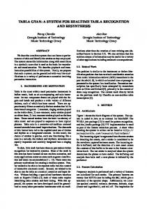
The INCR 2004 Algorithm. The author recently presented a practical incremental algorithm for maintaining the full distance matrix [8]. For ease of exposition, we shall refer to that algorithm as the INCR 2004 algorithm. That algorithm reduces the size of the network by collapsing all rigid components down to a single time-point.3 The INCR 2004 algorithm also reduces constraint propagation by propagating only along undominated edges.4 The undominated edges are stored in hash tables. In particular, for each time-point t, Precs(t) is a hash table containing the undominated edges coming in to t; and Succs(t) contains the undominated edges going out from t. The highlevel structure of the algorithm, which is based on work by several others [12, 13, 6], has two phases, called PropFwd and PropBkwd. The algorithm has time complexity O(k∆), where ∆ is the number of entries of D that actually need to be changed [12]. The PropFwd Phase. Suppose a new (or stronger) constraint, tj − ti ≤ δ, is added to the network. Fig. 1 illustrates the PropFwd phase, in which changes to distance matrix entries of the form, D(ti , t), are propagated by following the successors of tj . In the figure, decreasing the weight of the edge, ti tj , from 5 to 2 requires decreasing D(ti , tk ) from 9 to 6, and decreasing D(ti , tm ) from 17 to 14. Since D(ti , tp ) does not need to be changed, forward propagation stops at that point.5 During the PropFwd phase, each time-point, t, for which D(ti , t) changed is collected in a hash-table, AffectedTPs. The PropBkwd Phase. Fig. 2 illustrates the PropBkwd phase of the INCR 2004 algorithm. For each tm in AffectedTPs collected during the PropFwd phase, the predecessors of ti are followed, potentially leading to changes in entries of the form, D(t, tm ). For example, in the figure, the entry D(ti , tm ) had been reduced from 17 to 14 during the first phase. Its new value, requires reducing D(th , tm ) from 18 to 15. However, since D(tg , tm ) does not need to be changed, backward propagation stops at that point. Augmented STNs. An Augmented STN (ASTN) is an STN that has been augmented to include a special time-point, N, which repre3

4

5

N

−2

N

0 t 2

Z

A rigid component is a set of time-points in which the temporal distance between each pair of time-points is constrained to be some fixed value. Other researchers have described collapsing rigid components [17, 7]. A constraint is called undominated if removing it from the network would necessarily require updating the distance matrix. In contrast, removing a dominated constraint from the network would leave the distance matrix unchanged. The algorithm takes advantage of the fact that dominated constraints are easy to detect in networks with no rigid components [10]. For expositional simplicity, Fig. 1 shows only one branch of the sub-tree rooted at tj . The PropFwd phase normally explores multiple branches of that sub-tree. Similar remarks apply to the PropBkwd phase.

−3

After:

N

2

Z

direction of propagation Figure 2.

−1

t

−2

tm ti

tb tc

Figure 3.

During:

18

th 1

N 0

Figure 1. The PropFwd phase of the incremental algorithm

tg 6

0

−d

tp

tm

tk

4

ta

0

18

t

−2 Figure 4. The execution of the time-point t at time 2

sents the current time (i.e., “now”) [11]. Representing the now timepoint enables the network to explicitly handle the passage of time and the execution of time-points. The passage of time is handled by including a single edge from N to Z, with weight −d, representing the lower-bound constraint, d ≤ N. This edge, as illustrated in Fig. 3, is the only outgoing edge from the now time-point. As time passes, the value of d increases (i.e., the constraint involving Z and N grows stronger). Since the time-complexity of strengthening a constraint is lower than that of weakening or deleting constraints, this way of dealing with the passage of time is computationally attractive. In an ASTN, each unexecuted time-point, t, is constrained to occur at or after now—represented by an edge from t to N with weight 0. Fig. 3 illustrates these kinds of edges, which are the only incoming edges to the now time-point. When t is executed, the edge from t to N is deleted, and two edges between t and Z are inserted to fix t’s value. Fig. 4 provides “before”, “during” and “after” snapshots of a network in which t is executed at time 2. In the “before” snapshot, the current time is 1, and t is constrained to occur at or after that time. In the middle snapshot, t has been executed at time 2 (i.e., the edge from t to N has been deleted, and a pair of edges between t and Z have been inserted, fixing the value of t to 2). In the bottom snapshot, the current time has advanced to 3, but that has no effect on t. For an ASTN, the distance matrix entry, D(Z, N), can be interpreted as a kind of deadline [11]. In particular, if some time-point is not executed at or before this deadline, then the network is certain to become inconsistent—because the passage of time (i.e., the increased value of d on the edge from N to Z) will eventually generate a negative cycle. The potential inconsistency can be averted by executing one or more time-points, thereby deleting constraints involving N and increasing the value of D(Z, N).

2 Desiderata The main goal for the work described in this paper is to provide a temporal constraint management system that can serve as the basis for a temporal reasoning module in real-time planning, scheduling and acting applications, including multi-agent systems involving the coordination of temporally dependent, inter-agent activities. This high-level goal consists of the following subsidiary goals: • To maintain constant-time access to all distance-matrix entries • To reduce space requirements for the distance matrix (or any other auxiliary data structures)

ta

tb

ta

tb

5

5

8

8 −3

−2 Z

−3 −2

Zout

0

Zin

Figure 5. Replacing the zero time-point by a pair of time-points

• To reduce the need for constraint propagation • To include a fully dynamic constraint propagation algorithm that is scalable to real-time applications Constant-time access to distance-matrix entries facilitates multiagent coordination algorithms (e.g., temporal decoupling [9]). Reducing space requirements for the distance matrix implies not explicitly representing every distance-matrix entry, while maintaining constant-time access. Reducing the need for constraint propagation makes the fully dynamic algorithm computationally palatable. “Scalable” means that the resulting TCMS is practical for applications involving hundreds, or even thousands of time-points.

3 Approach This paper presents a TCMS called MYSYSTEM that meets the desiderata listed above. In MYSYSTEM: • The now time-point, N, is explicitly represented (as in ASTNs). • The zero time-point, Z, is replaced by a pair of time-points, Zin and Zout , thereby eliminating propagation through Z, and reducing the number of distance matrix entries needing to be computed. • Since the portion of the distance-matrix that is actually computed is typically quite small, the values are stored in a hash table, instead of a two-dimensional array. • The incremental algorithm is essentially the same as the INCR 2004 algorithm, except that rigid components and dominated constraints are handled differently. • A new decremental algorithm is provided that manipulates the same data structures as the incremental algorithm. The algorithm, which draws on ideas from other researchers [4, 13], is not the fastest possible, but requires only minor auxiliary data structures. • Executed time-points are effectively removed from the network. Replacing the Zero Time-Point by a Pair of Time-Points. In real-world applications, the starting and ending times of tasks are typically subject to a variety of unary constraints—that is, constraints involving the zero time-point, Z. As a result, while the maximum number of edges incident on any other time-point might be, say, ten, the number of edges incident on Z can be O(n). Thus, a great deal of the constraint propagation needed to fully populate the distance matrix is due to constraints involving Z. To eliminate constraint propagation through Z, the temporal network in MYSYSTEM replaces Z by a pair of time-points, Zin and Zout .6 In particular, as illustrated in Fig. 5, Zin is the destination for all edges that would normally point to Z, and Zout is the source of all edges that would normally emanate from Z. Now, adding an edge from Zin to Zout with weight 0 (shown as a dashed arrow in the figure) would make the two networks in Fig. 5 equivalent; however, such an edge is purposely left out of the network in MYSYSTEM. This seemingly minor change eliminates prop6

This treatment of the zero time-point is somewhat similar to Cesta and Oddi’s treatment of the zero time-point as both a source and a sink [2].

agation through Z; thus, it dramatically reduces the amount of computation required to maintain the distance matrix. At the same time, MYSYSTEM retains the property of having constant-time access to all distance-matrix entries. To see this, suppose A is a standard ASTN and A′ is the same as A, except that the zero time-point has been replaced by Zin and Zout , as described above. Because the edge from Zin to Zout is left out of A′ , the distance matrices, D and D′ , are typically quite different. However, the relationship between their corresponding entries is simple. In particular, for any ti , tj ∈ T \{Z}:7 • D(ti , Z) = D′ (ti , Zin ) • D(Z, tj ) = D′ (Zout , tj ) • D(ti , tj ) = min{D′ (ti , Zin ) + D′ (Zout , tj ), D′ (ti , tj )} The last equality can be glossed as: “The shortest path from ti to tj either involves the zero time-point or it doesn’t.” In this way, although D′ typically contains far fewer finite entries than D, it can be used to fetch the value of any entry in D(ti , tj ) in constant time. The Distance-Matrix Hash Table. Due to the use of Zin and Zout , the constraint propagation algorithms in MYSYSTEM typically need to compute only a small fraction of the O(n2 ) entries in the distance matrix, D′ . Thus, to save space, a hash table is used to store only those entries that are actually computed. Any entry, D′ (ti , tj ), that has not been stored in the hash table is taken to be infinity, representing that there is no path from ti to tj . Hash-table keys are integers of the form, N i + j, where N is an upper bound on the number of time-points in the network. 8 For example, if N = 214 = 16384, then 28-bit values can be used for hash-table keys—which can be quickly computed using left-shift and addition operations. A Note about Rigid Components and Undominated Edges. In a purely incremental context, constraints are never weakened or deleted. Thus, rigid components, once created, can never become non-rigid. Thus, it is safe to collapse each rigid component down to a single point as soon as it is created. Insodoing, the network remains free from rigidities, which simplifies the detection of dominated constraints. In contrast, a fully dynamic algorithm must handle the weakening or deleting of constraints and, thus, cannot afford to collapse all rigid components—because undoing such transformations can be too computationally costly. Thus, the fully dynamic algorithm in MYSYSTEM does not typically collapse rigid components. Thus, the network in MYSYSTEM may contain rigidities, thereby complicating the detection of dominated edges. For this reason, the detection of dominated edges in MYSYSTEM is restricted to cases where a strictly shorter alternative pathway is found.9 In addition, the decremental algorithm can sometimes insert dominated edges into the Precs and Succs hash tables—because avoiding doing so would be too computationally costly. However, when the incremental algorithm detects these dominated edges, they are immediately removed from the Precs and Succs hash tables. Thus, in this sense, the fully dynamic algorithm in MYSYSTEM can be said to propagate along “mostly” undominated edges. The Decremental Algorithm in MYSYSTEM. The decremental algorithm is used when an existing constraint, tj − ti ≤ δ, is either weakened or deleted. The algorithm has the following three phases: (1) In a hash-table called Changelings, collect all pairs, (tx , ty ), such that D′ (tx , ty ) might need updating. 7 8 9

T \{Z} denotes the set of time-points in A other than Z. Demetrescu and Italiano [4] encode pairs in this way. In contrast, the INCR 2004 algorithm also detects edges that are dominated by a path whose length is the same as that of the edge being dominated.

(2) For each (tx , ty ) in Changelings, check for shorter alternative pathways from tx to ty ; collect the shortest alternatives in a hash-table called AltPaths. (3) Incrementally propagate the constraints in AltPaths. Phase 1. Consider the path from tx to ty shown below, where the wavy arrows represent shortest paths and δ is the original weight of the edge being weakened/deleted.

tx

ti

δ

tj

ty

The pair, (tx , ty ), is collected during Phase 1 if and only if: D′ (tx , ty ) = D′ (tx , ti ) + δ + D′ (ti , ty ) All such pairs are collected using a two-pass algorithm that has the same structure as the PropFwd and PropBkwd phases of the incremental algorithm. Thus, Phase 1 takes time O(k∆), where ∆ is the number of pairs in Changelings. After the Changelings hash-table has been populated, the corresponding distance-matrix entries are assigned new values, as follows. If the edge, ti tj , has been deleted, then each D′ (tx , ty ) is set to ∞, because the deletion of ti tj might mean there no longer is any path from tx to ty . On the other hand, if ti tj was simply weakened—say by an amount α—then each D′ (tx , ty ) is set to the value D′ (tx , ty ) + α + 1. Using this value, which is necessarily greater than the eventual updated value, forces D′ (tx , ty ) to be updated during Phase 2 or 3. Since MYSYSTEM does not maintain any pointers to first or last steps of shortest paths (e.g., as done by Rohnert [13]), the Changelings hash table may end up containing some pairs whose distance-matrix entries do not need to be updated. Instead of maintaining complex auxiliary data structures to avoid this, the decremental algorithm discovers alternative paths during Phase 2 and 3 to ensure that the corresponding distance-matrix entries are restored. Phase 2. For each (tx , ty ) in Changelings, alternative pathways of the forms given below are collected in a hash-table called AltPaths.10 tx

ty

edge

tx

tk

ty

shortest path

edge

tx

tv shortest path

ty edge

For some (tx , ty ) in Changelings, it may be that no alternative paths exist. For other pairs, more than one such path may exist; however, only the shortest such paths are kept in AltPaths. The hash-key for the AltPaths hash table is the pair, (tx , ty ); the value is the length of the alternative path. (Interior time-points on the path are not needed.) Notice that the alternative pathways collected during Phase 2 may well have been dominated prior to the weakening (or deleting) of the edge ti tj , as illustrated below in the case of an alternative edge. 16

tx 3

ti

5

ty tj

4

Prior to weakening ti tj from 5 to 10, the edge, tx ty was not a shortest path; however, afterward, it becomes a shorter (and possibly shortest) 10

Demetrescu and Italiano [4] refer to such pathways as locally shortest.

path. For this reason, the edges considered during Phase 2 are drawn from the set C—which contains all of the edges in the network—not just those in the Precs and Succs hash tables. Phase 3. During Phase 3, the alternative paths found in Phase 2 are incrementally propagated. There are several options for doing this. Each alternative path could, in turn, be completely propagated using the incremental algorithm. However, this sort of depth-first approach might result in a large amount of redundant propagation. Another option, analogous to A∗ search, would be to sort the alternative paths according to how close their path-lengths were to the original value of D′ (tx , ty ) and apply the incremental algorithm to those alternative paths in their sorted order. The decremental algorithm in MYSYSTEM takes an iterative, breadth-first approach. In the first iteration, each path in AltPaths is propagated only one step along the predecessors of tx and the successors of ty . Each one-step propagation generates a new update which is stored in a hash-table called newAltPaths. During the second iteration, each update in newAltPaths is propagated only one step, generating new updates for the third iteration. This iterative process terminates when no more updates are generated. Empirical evidence suggests that this form of incremental propagation is quite practical. Removing Executed Time-Points. As discussed earlier, the fully dynamic algorithm does not typically collapse rigid components, because undoing such transformations in response to constraint relaxations can be too computationally costly. However, when a timepoint, t, is executed, it forms a rigid component with Zin and Zout that is guaranteed to persist. Thus, it is safe to collapse this kind of rigid component. Doing so effectively removes t from the network by reorienting constraints involving t toward Zin and Zout .

4 Empirical Evaluation The MYSYSTEM TCMS was tested on a set of thirty 25-agent scheduling problems drawn from the Phase 2 Evaluation for the DARPA Coordinators Project [15]. These kinds of problems are represented in the cTAEMS language, the details of which are described elsewhere [1]. The important characteristics of the test problems are shown in the top plot in Fig. 6. Each problem involved between 1507 and 3273 time-points (plotted on the horizontal axis) and between 803 and 1686 activities (ACTS).11 For each problem, a centralized scheduler [14] was used to generate a set of agent schedules seeking to optimize the cTAEMS quality metric. In the process, the scheduler invoked the incremental algorithm of MYSYSTEM between 3461 and 7353 times (INCRS), and the decremental algorithm between 254 and 1185 times (DECRS). The resulting schedules included a total of between 139 and 243 activities (SCHEDS), and resulted in networks with between 3326 and 6797 edges (EDGES). The middle plot of Fig. 6 shows the CPU time used by MYSYSTEM to do all of the temporal computations for each scheduling problem. The CPU time ranged from 2 seconds to 2 minutes for each problem. In the worst case, the 2 minutes of computation, spread over 8000 invocations of the incremental or decremental algorithms, averaged to about 15 msec per invocation. The bottom plot of Fig. 6 shows the memory usage by MYSYS TEM . The number of finite distance-matrix cells (i.e., those that were actually stored in a hash table) ranged from about 77,000 to about 850,000 per problem. In contrast, the full distance matrix would have required between 2.2 and 10.7 million cells. Given that typical entries are four bytes, such a matrix could have required over 40 megabytes 11

Some activities share time-points; hence the number of time-points is somewhat less than double the number of activities.

INCRS 7000

EDGES

5000

3000

Acknowledgments ACTS

1000

DECRS SCHEDS 1600

2000

2400

2800

3000

NUMBER OF TIME POINTS

3

CPU SECONDS

10

1

10

0

1600

2000

2400

2800

3000

NUMBER OF TIME POINTS

8

10

Total Memory Used (Bytes)

7

10 Potential Size of Distance Matrix 6

10

5

10

Number of Finite Distance Matrix Entries

4

10

The research presented in this paper was supported in part by subcontract 55-000723 between Vassar College and SRI International as part of the DARPA Coordinators Project (Contract FA8750-05-C0033). Any opinions, findings and conclusions or recommendations expressed in this paper are those of the author and do not necessarily reflect the views of DARPA. The author thanks Stephen Smith, Zachary Rubinstein, Terry Zimmerman, Laura Barbulescu and Anthony Gallagher from Carnegie Mellon University for providing access to their scheduler.

REFERENCES

2

10

10

tries that typically need to be computed. The fully dynamic algorithm extends an earlier incremental algorithm. It limits propagation to “mostly” undominated edges. The paper provided empirical results on temporal networks derived from a centralized scheduler applied to a variety of 25-agent scheduling problems involving thousands of time-points.

1600

2000

2400

2800

3000

NUMBER OF TIME POINTS

Figure 6.

Results of experiments on 25-agent scheduling problems

of memory. In contrast, the total memory used by MYSYSTEM during the course of each scheduling problem, most of which was dynamically allocated and freed, ranged from about 8 to 92 megabytes. All experiments were run on an IBM Thinkpad laptop with a 2.4GHz Intel processor using Allegro Common Lisp, version 8.1.

5 Conclusion This paper presented a new temporal constraint management system, called MYSYSTEM, that combines novel STN representations with a fully dynamic propagation algorithm that is practical for realworld, real-time applications. The temporal network in MYSYSTEM includes special time-points to eliminate a common form of constraint propagation and reduce the number of distance-matrix en-

[1] M. Boddy, B. Horling, J. Phelps, R. Goldman, R. Vincent, C. Long, and B. Kohout, ‘C taems language specification, version 1.06 (0)’. [2] Amedeo Cesta and Angelo Oddi, ‘Gaining efficiency and flexibility in the simple temporal problem’, in Proceedings of the Third International Workshop on Temporal Representation and Reasoning (TIME-96), pp. 45–50. IEEE, (1996). [3] Rina Dechter, Itay Meiri, and Judea Pearl, ‘Temporal constraint networks’, Artificial Intelligence, 49, 61–95, (1991). [4] C. Demetrescu and G. Italiano, ‘A new approach to dynamic all pairs shortest paths’, in Proceedings of the 35th STOC, pp. 159–166, (2003). [5] Camil Demetrescu and Giuseppe F. Italiano, ‘Improved bounds and new trade-offs for dynamic all pairs shortest paths’, Technical Report ALCOMFT-TR-02-1, ALCOM, (2002). [6] Shimon Even and Hillel Gazit, ‘Updating distances in dynamic graphs’, Methods of Operations Research, 49, 371–387, (1985). [7] Alfonso Gerevini, Anna Perini, and Francesco Ricci, ‘Incremental algorithms for managing temporal constraints’, Technical Report IRST9605-07, IRST. [8] Luke Hunsberger, ‘Quantitative temporal reasoning in planning problems’. AAAI-2004 Tutorial MP-2, slides available at: http://www.cs.vassar.edu/˜hunsberg. [9] Luke Hunsberger, ‘Algorithms for a temporal decoupling problem in multi-agent planning’, in Proceedings of the Eighteenth National Conference on Artificial Intelligence (AAAI-2002), (2002). [10] Luke Hunsberger, Group Decision Making and Temporal Reasoning, Ph.D. dissertation, Harvard University, 2002. Available as Harvard Technical Report TR-05-02. [11] Luke Hunsberger, ‘Distributing the control of a temporal network among multiple agents’, in Proc. of the 2nd Int’l. Joint Conference on Autonomous Agents and MultiAgent Systems (AAMAS-03), (2003). [12] G. Ramalingam and Thomas Reps, ‘On the computational complexity of dynamic graph problems’, Theoretical Computer Science, 158, 233– 277, (1996). [13] Hans Rohnert, ‘A dynamization of the all pairs least cost path problem’, in 2nd Symposium of Theoretical Aspects of Computer Science (STACS 85), ed., Kurt Mehlhorn, volume 182 of Lecture Notes in Computer Science, 279–286, Springer, (1985). [14] S. Smith, A.T. Gallagher, T.L. Zimmerman, L. Barbulescu, and Z. Rubinstein, ‘Distributed management of flexible times schedules’, in Intl. Conf. on Autonomous Agents and Multiagent Systems, (2007). [15] Valerie Guralnik Thomas Wagner, John Phelps and Ryan VanRiper, ‘COORDINATORS: Coordination managers for first responders’, in Proc. of the 3rd Intl. Joint Conference on Autonomous Agents and Multiagent Systems (AAMAS-2004). IEEE Computer Society, (2004). [16] Mikkel Thorup, ‘Worst-case update times for fully-dynamic all-pairs shortest paths’, in Annual ACM Symposium on Theory of Computing, pp. 112–119, (2005). [17] Ioannis Tsamardinos, Reformulating Temporal Plans for Efficient Execution, Master’s thesis, University of Pittsburgh, 2000.