A precise calculation of power system frequency and phasor - Power ...

494

IEEE TRANSACTIONS ON POWER DELIVERY, VOL. 15, NO. 2, APRIL 2000

A Precise Calculation of Power System Frequency and Phasor Jun-Zhe Yang and Chih-Wen Liu

Abstract—A series of precise digital algorithms based on Discrete Fourier Transforms (DFT) to calculate the frequency and phasor in real-time are proposed. These algorithms that we called the Smart Discrete Fourier Transforms (SDFT) family not only keep all of the advantages of DFT but also smartly take frequency deviation, and harmonics into consideration. These make the SDFT family more accurate than the other methods. Besides, SDFT family is recursive and very easy to implement, so it is very suitable for use in real-time. We provide the simulation results compared with conventional DFT method and second-order Prony method to validate the claimed benefits of SDFT. Index Terms—Discrete Fourier Transforms (DFT), Frequency estimation, phasor measurement.

the advantages that it can obtain exact solution in the presence of harmonics and frequency deviation from nominal frequency. The organization of this paper is as follows: We describe basic principle of SDFT in section II. DFT, Prony method and SDFT are tested by four examples in section III. Finally, we give a conclusion in section IV. II. THE PROPOSED DIGITAL ALGORITHM This section presents the algorithm of the basic SDFT that estimates the frequency and phasor from a voltage/current signal. Consider a sinusoidal input signal of frequency ! = 2f as follows:

x(t) = X

I. INTRODUCTION

F

REQUENCY and phasor are the most important quantities in power system operation because they can reflect the whole power system situation. Frequency can show the dynamic energy balance between load and generating power, while phasor can constitute the state of system. So frequency and phasor are regarded as indices for the operating power systems in practice. However, utilities have difficulty in calculating those quantities precisely. There are many devices, such as power electronic equipment and arc furnaces, etc. generating lots of harmonics and noise in modem power systems. It is therefore essential for utilities to seek and develop a reliable method that can measure frequency and phasor in presence of harmonics and noise. With the advent of the microprocessor, more and more microprocessor-based equipments have been extensively used in power systems. Using such equipment is known to provide accurate, fast responding, economic, and flexible solutions to measurement problems [1]. Therefore, all we have to do is to find the best algorithm and implement it. There have been many digital algorithms applied to calculating frequency or phasor during recent years, for example Modified Zero Crossing Technique [2], Level Crossing Technique [3], Least Squares Error Technique [4]–[6], Newton method [7], Kalman Filter [8], [9], Prony Method [10], and Discrete Fourier Transform (DFT) [11], etc. For real-time use, most of the aforementioned methods have trade-off between accuracy and speed [12]. Unlike other methods, a series of precise digital algorithms, namely Smart Discrete Fourier Transform (SDFT) family, are presented and tries to meet the real-time use. SDFT family has Manuscript received February 4, 1999. The authors are with the Department of Electrical Engineering, National Taiwan University, Taipei, Taiwan. Publisher Item Identifier S 0885-8977(00)03461-0.

cos(!t +

)

(1)

where X : the amplitude of the voltage/current signal, : the phase angle of the voltage/current signal Suppose that x(t) is sampled with a sampling rate (603 N ) Hz waveform to produce the sample set fx(k)g

x(k) = X



cos

k ! 60N



k = 0; 1; 2; 1 1 1 ; N 0 1:

+

(2) The signal x(t) is conventionally represented by a phasor (a complex number) x x = Xej = X cos  + jX sin : (3) Then x(t) can be expressed as xej!t + x3 e0j!t

x(t) =

2

(4)

where 3 denotes complex conjugate. Moreover, the fundamental frequency (60Hz) component of DFT of fx(k)g is given by N 01 2 X 2k x^r = x(k + r)e0j N : (5) N k=0 Combing Eq. (4) and Eq. (5) and taking frequency deviation !  f into consideration, at last, we obtain:

( = 2 (60 + 1 )) N 1  x sin 2 x ^r = N ej 60N (1f (2r+N01)+120r) 1 sin 2 N 2 x3 sin 2  +N e0j 60N (1f (2r+N01)+120(r+N01)) sin 22

0885–8977/00$10.00 © 2000 IEEE

Authorized licensed use limited to: National Taiwan University. Downloaded on March 9, 2009 at 04:14 from IEEE Xplore. Restrictions apply.

(6)

YANG AND LIU: A PRECISE CALCULATION OF POWER SYSTEM FREQUENCY AND PHASOR

= 2601Nf ;

1

Moreover, we can estimate phasor after getting exact “f ” by the following equations:

 1 f 2 2 + 60 : 2 = N 

where and

495

Ar

If we define Ar and Br as Ar

Br

=

=

x N

N 1

sin 2 sin 21

 ej 60N (1f (2r +N 01)+120r)

sin N22 0j  (1f (2r+N 01)+120(r+N 01)) : e 60N 2 sin 2

x3 N

X

(7)

(8)

^ = Ar + Br :

(9)

Actually, the first half development of the algorithm of SDFT is the same as the conventional DFT method. So the SDFT can keep all advantages of DFT such as recursive computing manner. In the conventional DFT, it assumes that the frequency deviation is small enough to be ignored, and xr  Ar . Therefore,

^

= arctan(imag(^xr )=real(^xr )) r 0 r01 f = 60 + 2 2 60N:

r

= ej( 60N (21f +120)):

Then

( ) = X1 cos(!t + 1) + X2 cos(m!t + 2)

X1 ; X2 : the amplitude, 1 ; 2 : the phase angle.

Following similar steps developed previously, we can get:

2

1f )r NX 01 j 2 1f k 60 60N x ^r = e k=0 2  1 f N 01 3 X x 0j (1+ + N e N 60 )r k=0 1 f (2 + 60 ) 0j 2 k N 2e 2 1f NX 01 + Nx ej N (1+ 60 )mr k=0 m1f (m 0 1 + 60 ) j 2 k N 2e 2 1f )mr NX 01 x3 0j (1+ + N e N 60 k=0 m1f (01 0 m + 60 ) 0j 2 k  (1+ x j N e N

(12)

= Ar+1 + Br+1 = Ar 3 a + Br 3 a01

(15)

^

xr+2

= Ar+2 + Br+2 = Ar+1 3 a + Br+1 3 a01 = Ar 3 a2 + Br 3 a02:

(16)

(14)

There are three unknown variables in Eq. (9), Eq. (15) and Eq. (16), and after some algebraic manipulations we obtain:

^ 3 a2 0 (^xr + x^r+2) 3 a + x^r+1 = 0:

xr+1

Solve Eq. (17) to obtain

(17)

q

(^xr + x^r+2) 6 (^xr + x^r+2)2 0 4^x2r+1 a= : 2^xr+1 Then from the definition of “a” in Eq. (12), we can get the exact solution of the frequency f

= 60 + 1f = cos01(Re(a)) 3 602N :

(18)

(22)

where

(11)

(13)

^

(20)

x t

(10)

= Ar 3 a = Br 3 a01:

xr+1

3 sin 60N  1f 

deviation. Next, we take harmonics into consideration. Assume a sinuf with mth harmonic given soidal signal of frequency ! by:

And from Eq. (7) and Eq. (8), we will find the following relations Ar+1 Br+1

N

sin 60   = angle(Ar ) 0 60N 2 (1f 2 (N 0 1)): (21) It is observed that SDFT can provide exact frequency and ^r , x^r+1 and x^r+2 in the presence of frequency phasor using x

Conventional DFT methods incur error in estimating frequency and phasor when frequency deviates from nominal frequency (60Hz). However, in the SDFT we take Br into consideration. So we define a

= abs(Ar ) 3

(19)

 1f 

=2

Then Eq. (6) can be expressed as xr

= x^r+1a230a 10 x^r

2e

N

:

(23)

Then

^ =

xr

x1 N

sin N21 j(=60N )(1f (2r+N 01)+120r) e sin 21

+

x31 N

+

x2 N

sin N22 0j(=60N )(1f (2r+N 01)+120(r+N 01)) e sin 22 sin N23 sin 23

Authorized licensed use limited to: National Taiwan University. Downloaded on March 9, 2009 at 04:14 from IEEE Xplore. Restrictions apply.

496

IEEE TRANSACTIONS ON POWER DELIVERY, VOL. 15, NO. 2, APRIL 2000

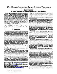
Fig. 1. Test signal: v (t) = cos(!t); simulated frequency 59.5 Hz; sampling frequency 960 Hz.

2 ej (=60N )(m1f (2r +N 01)+60(2mr+mN 0m0N +1)) 3 + x2 N

 1 2 m 0 1 + 60 ; 3 = N 

sin N24 sin 24

2 e0j (=60N )(m1f (2r+N 01)+60(2mr+mN 0m +N 01))

and

(24)

^ = Ar + Br + Cr + Dr

xr

^

xr+1

= Ar+1 + Br+1 + Cr+1 + Dr+1 = Ar 3 a + Br 3 a01 + Cr 3 am + Dr 3 a0m

(25)

(26)

Cr

=

sin N23 sin 23

2 e0j (=60N )(m1f (2r+N 01)+60(2mr+mN 0m0N +1)) Dr

=

x32 N

sin N24 sin 24

2 e0j (=60N )(1f (2mr+N 01)+60(2mr+mN 0m+ N 01))

=

  m1f 2 0m 0 1 + 60 N

:

There are five unknown variables in Eq. (25), hence, we need five equations to solve this problem. So using xr , xr+1 , xr+2 , xr+3 and xr+4 , we can get exact frequency and phasor in the presence of one harmonic. We use SDFT, to denote that 3rd harmonic has been taken into consideration. Of course, any other integral order harmonic can be taken into consideration too, for example: SDFT35 and SDFT357 take 3rd , 5th harmonic and 3rd , 5th , 7th harmonic into consideration respectively. Similarly, nonintegral harmonics also can be developed. We use SDFTn to denote that nonintegral harmonics has been taken into consideration.

^

where x2 N

4

m f

^ ^

^

^

III. SIMULATION RESULTS Most of the frequency estimation methods are concerned with the performances of the four cases: frequency deviation, frequency variation, harmonics and noise. Hence, we used these four cases to compare the performance of these methods. Simulation results presented in this section were all simulated from

Authorized licensed use limited to: National Taiwan University. Downloaded on March 9, 2009 at 04:14 from IEEE Xplore. Restrictions apply.

YANG AND LIU: A PRECISE CALCULATION OF POWER SYSTEM FREQUENCY AND PHASOR

497

Fig. 2. Test signal: v (t) = cos(!t); simulated frequency variation form 59.5 Hz to 60.5 Hz during 1 second; sampling frequency 960 Hz.

Fig. 3. Test signal: v (t) = cos(!t); simulated frequency variation like sin wave during 1 second; sampling frequency 960 Hz.

Matlab and shown for a fair comparison to DFT method and Prony method. In Fig. 1(a), we showed that SDFT family and the Prony method could obtain an exact frequency calculation under frequency deviation in a pure sinusoidal waveform. We also

show the performance of conventional DFT method. It is clear that conventional DFT method gives the wrong answer in frequency and phasor. By comparison of computation speed, Fig. 1(d) shows the AMD K6-200 CPU time of each method. There are 960 data per second computed by each method.

Authorized licensed use limited to: National Taiwan University. Downloaded on March 9, 2009 at 04:14 from IEEE Xplore. Restrictions apply.

498

IEEE TRANSACTIONS ON POWER DELIVERY, VOL. 15, NO. 2, APRIL 2000

Fig. 4. Test signal: v (t) = cos(!t) + 0:05 cos(3!t) + 0:02 cos(5!t) + O:O1 cos(7!t); simulated frequency 60.05 Hz; sampling frequency 960 Hz.

Fig. 5. Test signal: v (t) = cos(!t); simulated frequency 60 Hz; sampling frequency 960 Hz; with 1% noise.

In Fig. 2 and Fig. 3, we put the emphasis on the frequency variation. The frequency of test signal in Fig. 2 is varied linearly form 59.5 Hz to 60.5 Hz during 1 second. Another test in Fig. 3 is

to make the frequency change like a sinusoid: f =60+ sin(2t). It is observed that the errors of conventional DFT method are larger than SDFT family in terms of frequency and phasor.

Authorized licensed use limited to: National Taiwan University. Downloaded on March 9, 2009 at 04:14 from IEEE Xplore. Restrictions apply.

YANG AND LIU: A PRECISE CALCULATION OF POWER SYSTEM FREQUENCY AND PHASOR

We designed the test frequency to be 60.05Hz and added 3rd , and 7th harmonics into test signal in Fig. 4. In Fig. 4a, we find that Prony method is very sensitive to harmonic. Although Prony method can change its window size, it still can’t have better performance. SDFT has better performance than DFT, and the rest of SDFT family, expect SDFTn , is better than SDFT. SDFT357 , SDFT35n and SDFT357n get the exact frequency and phasor in this case. We know that if a method can be used in real world, it must take noise into consideration. The frequency of test signal in Fig. 5 is 60Hz, and we add one percent of white noise into signal. In Fig. 5, we didn’t show the performance of Prony Method, since the performance of Prony method depends on window size in this test. It is shown that SDFT is better than DFT and SDFT357n is better than SDFT.

5th

IV. CONCLUSION In this paper we introduce the SDFT family and demonstrate their performance. SDFT family both keeps the advantages of DFT and also deals with the difficulty of frequency deviation errors, while taking harmonics, noise into consideration. These aspects make SDFT family accurate, harmonic-resisting methods. If only rough answer is required, DFT is still a good choice, but if precise answer is essential, we recommend SDFT family. We believe that SDFT family has a great potential to replace conventional DFT method for power system frequency and phasor calculation in the future, if SDFT family can be speeded up by the advanced computing architecture. REFERENCES [1] P. J. Moore, R. D. Carranza, and A. T. Johns, “Model System Tests on a New Numeric Method of Power System Frequency Measurement,” IEEE Transactions on Power Delivery, vol. 11, no. 2, pp. 696–701, Apr. 1996. [2] Miroslav M. Begovic, Petar M. Djuric, Sean Dunlap, and Arun G. Phadke, “Frequency Tracking in Power Networks in the Presence of Harmonics,” IEEE Transactions on Power Delivery, vol. 8, no. 2, pp. 480–486, Apr. 1993. [3] C. T. Nguyen and K. Srinivasan, “A New Technique for Rapid Tracking of Frequency Deviations Based on Level Crossings,” IEEE Transactions on Power Apparatus and Systems, vol. PAS-103, no. 8, pp. 2230–2236, Aug. 1984.

499

[4] I. KAMWA and R. GRONDIN, “Fast Adaptive Schemes for Tracking Voltage Phasor and Local Frequency in Power Transmission and Distribution Systems,” IEEE Transactions on Power Delivery, vol. 7, no. 2, pp. 789–795, Apr. 1992. [5] M. S. Sachdev and M. M. Giray, “A Least Error Squares Technique for Determining Power System Frequency,” IEEE Transactions on Power Apparatus and Systems, vol. PAS-104, no. 2, pp. 437–443, Feb. 1985. [6] M. M. Giray and M. S. Sachdev, “Off-Nominal Frequency Measurements in Electric Power Systems,” IEEE Transactions on Power Delivery, vol. 4, no. 3, pp. 1573–1578, July 1989. [7] Vladimir V. Terzija, Milenko B. Djuric, and Branko D. Kovacevic, “Voltage Phasor and Local System Frequency Estimation Using Newton Type Algorithm,” IEEE Transactions on Power Delivery, vol. 9, no. 3, pp. 1368–1374, July 1994. [8] M. S. Sachdev, H. C. Wood, and N. G. Johnson, “Kalman Filtering Applied to Power System Measurements for Relaying,” IEEE Transactions on Power Apparatus and System, vol. PAS-104, no. 12, pp. 3565–3573, Dec. 1985. [9] Adly A. Girgis and William L. Peterson, “Adaptive Estimation of Power System Frequency Deviation and its Rate of Change for Calculating Sudden Power System Overloads,” IEEE Transactions on Power Delivery, vol. 5, no. 2, pp. 585–594, Apr. 1990. [10] Tadusz Lobos and Jacek Rezmer, “Real-Time Determination of Power System Frequency,” IEEE Transactions on Instrumentation and measurement, vol. 46, no. 4, pp. 877–881, Aug. 1997. [11] A. G. Phadke, J. S. Thorp, and M. G. Adamiak, “A New Measurement Technique for Tracking Voltage Phasors, Local System Frequency, and Rate of Change of Frequency,” IEEE Transactions on Power Apparatus and Systems, vol. 102, no. 5, pp. 1025–1038, May 1983. [12] Ph. Denys, C. Counan, L. Hossenlopp, and C. Holweck, “Measurement Of Voltage Phase For The French Future Deffence Plan Against Losses Of Synchronism,” IEEE Transactions on Power Delivery, vol. 7, no. 1, pp. 62–69, Jan. 1992.

Jun-Zhe Yang was born in Taiwan in 1971. He received his B.S. degree in electrical engineering from Tatung Institute of Technology in 1992 and M.S. degree from National Taiwan University in 1995. He is presently a graduate student in the electrical engineering department, National Taiwan University, Taipei, Taiwan.

Chih-Wen Liu was born in Taiwan in 1964. He received the B.S. degree in Electrical Engineering from National Taiwan University in 1987, and M.S. and Ph.D. degrees in electrical engineering from Cornell University in 1992 and 1994. Since 1994, he has been with National Taiwan University, where he is associate professor of electrical engineering. He is a member of the IEEE and serves as a reviewer for IEEE TRANSACTIONS ON CIRCUITS AND SYSTEMS, PART I. His main research area is in application of computer technology to power system monitoring, operation, protection and control. His other research interests include GPS time transfer and chaotic dynamics and their application to system problems.

Authorized licensed use limited to: National Taiwan University. Downloaded on March 9, 2009 at 04:14 from IEEE Xplore. Restrictions apply.