A Preliminary Study of LORAN-C Additional

Presented at ILA-31, Washington DC, 28-30 October 2002

A Preliminary Study of LORAN-C Additional Secondary Factor (ASF) Variations CAPT Richard Hartnett, PhD, US Coast Guard Academy Gregory Johnson, JJMA, Inc. Peter F. Swaszek, PhD, University of Rhode Island Mitchell J. Narins, US Federal Aviation Administration

Abstract Currently, there is considerable interest in the LORAN community in the recognition of LORAN-C as “the” backup navigation system for the global positioning system (GPS). A key to this recognition is the demonstration to aviation navigation that LORAN-C can achieve the accuracy, availability, integrity, and continuity to support non-precision approaches (RNP 0.3). To do so, it is required that we better understand the variations in the LORAN position “fix” due to the changing characteristics of the signal propagation path (so called additional secondary factors or ASFs). The U.S. Coast Guard Academy, under contract to the Federal Aviation Administration (FAA), is attempting to understand and characterize these variations for “all-inview” receivers using time-of-arrival (TOA) data. This paper reports on some recent results in this arena.

Introduction The Federal Aviation Administration (FAA) observed in its recently completed Navigation Transition Study that LORAN-C, as an independent radionavigation (RNAV) system, is theoretically the best backup for the Global Positioning System (GPS). However, the FAA also observed that LORAN-C’s potential benefits to aviation hinges upon its ability to support nonprecision approach (NPA), which equates to a Required Navigation Performance (RNP) of 0.3. The tests and evaluations the FAA is conducting and sponsoring will determine whether LORAN-C can provide the accuracy, availability, integrity, and continuity to support NPA. A key component in these evaluations is a better understanding of ASFs and how to apply them to achieve more accurate LORAN-C positions while ensuring that the possibility of providing hazardous and misleading information (HMI) will be no greater than 1 x 10-7. The U.S. Coast Guard Academy, as a part of the FAA’s Government, Industry, and Academic team, is striving to improve our understanding of both the temporal and spatial variations in time of arrival (TOA) that could be mitigated through use of appropriate additional secondary factors (ASFs) [4,5,9,10,11]. Flight tests conducted jointly with Ohio University in August 2002 employed a digital downconverter (DDC)-based LORAN-C receiver to collect LORAN position data concurrent with a Novatel OEM-4 GPS receiver to collect WAAS GPS positions. A PC-104-form factor LORANC receiver utilizing an H-field antenna was used to collect TOA ASF data while the aircraft sat on the ground in the vicinity of the intended flight. During post-processing of the recorded flight data, ideal ASFs were applied to the TOAs recorded during the flight to determine a corrected LORAN position. The WAAS GPS derived positions were used as “truth” to compute the

1

Presented at ILA-31, Washington DC, 28-30 October 2002

“error” in each LORAN provided position. These position errors were then plotted geographically to show the position error as a function of distance from the ASF calibration point which gives some insight into the spatial variation of the ASFs. This paper presents preliminary results on characterizing the spatial variations in ASF corrections. Other results include validation of the data collection methodology and equipment and specification of the required data and formats. Plans for future testing and analysis to enable compilation and validation of an initial ASF database are also provided.

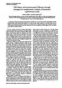
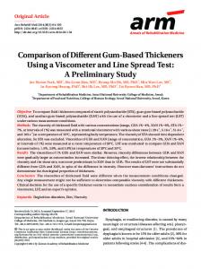
Methodology of Data Collection The Coast Guard Academy developed PC-104 H-field LORAN receiver [1, 7, 8] was used as the primary component of the ASF data collection system. A block diagram of the overall system is below in Figure 1. The receiver itself is implemented in an industry standard PC-104 form-factor and consists of 3 PC-104 boards – a Gatefield board, a CPU board, and an oscillator board – that are stacked together (see the photograph in Figure 2). Inputs to the PC-104 receiver are the two RF channels from the H-field antenna, a GPS 1 PPS (pulse per second) signal for the timing reference, and a 12.8 MHz clock signal from a stable signal source. In this case a DS-345 Function Generator that has been stabilized with a 10 MHz reference from a cesium oscillator.

1 PPS

Novatel OEM-4 WAAS GPS

H-field antenna

10 MHz

PC-104 Rcvr

DS-345 12.8 MHz

2 Channels RF

Save to disk: TIC, RAW TOA, ECD, SNR, etc.

Figure 1 – Block diagram of ASF data collection system.

2

Presented at ILA-31, Washington DC, 28-30 October 2002

Figure 2 – Picture of USCGA PC-104 LORAN Receiver The general procedure to collect ASF measurements is to run the PC-104 receiver in the location for which the ASF’s are desired. The latitude and longitude of the location need to be known very accurately. In practice a DGPS or WAAS GPS receiver is used to collect positions over a period of time at the location. The actual position is taken to be the average of these position samples. The PC-104 receiver can only track 3 chains simultaneously (a limitation of the Gatefield board), so ASF corrections can only be calculated for stations in those 3 chains. The receiver saves the TIC (time interval count), and the RAW TOA for each station at user configurable intervals; typically 2 seconds. The receiver also saves the tracking point strength, the SNR, and the ECD for each station as well as calculated latitude and longitude, time, and heading. This data file is then post-processed using the calibrated location of the receiver (as determined from DGPS/WAAS GPS). The timing relationships, and how the ASF is derived from this information is illustrated in Figure 3 on the next page.

3

Presented at ILA-31, Washington DC, 28-30 October 2002

Emission Delay Correction

Master Xmit (Master offset from 1 PPS) mod 200 µsec = 0

Station Xmit Emission Delay

Time Interval Counter

1 PPS

Predicted all seawater path TOA

Raw TOA

PCI Strobe

ASF

Loran signal rcvd Receiver Delay

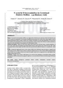
Figure 3 – ASF definition. Using the following definitions: TIC (time interval counter) = time interval from 1 PPS pulse to start of PCI. Raw TOA = time interval from start of PCI to when the receiver thinks the signal is received. Master offset = time interval from 1 PPS pulse to when the Master transmits. The Master station is nominally synchronized to this so that Master offset mod 200 microseconds = 0. Receiver (Rcvr) Delay = time delay introduced by receiver due to analog front end as well as digital filtering. ED = published Emission Delay for the Secondary station. EDC = Emission Delay Correction = difference from when the Secondary should have transmitted based upon the ED and when the Secondary actually transmits, referenced to 1 PPS. TOA = Time of Arrival = propagation time from Secondary (known position) to receiver (calibrated position) assuming an all-seawater propagation path. ASF = Additional Secondary Factor = propagation time adjustment due to the fact that the path is not all-seawater and the diagram above (Figure 3), it is clear that: TIC + Raw TOA - Rcvr Delay = Master offset + ED + EDC + TOA + ASF Of these values, EDC and ASF are those that contribute to position error. Solving for these two error terms: ASF + EDC = TIC + Raw TOA - Rcvr Delay - Master offset - ED - TOA Now, taking each side modulo 200 microseconds, we are left with: ASF + EDC = (TIC + Raw TOA - Rcvr Delay - ED - TOA) mod 200 since Master offset mod 200 = 0 and ASF and EDC are both