Since the relative motion of I in the camera coordinate system is. (dxi /dt, dyi /dt, dzi /dt) = âV â I ..... (optical flow) was then taken as the input to the model, and the.
Computer Vision and Image Understanding Vol. 76, No. 3, December, pp. 205–212, 1999 Article ID cviu.1999.0798, available online at http://www.idealibrary.com on
A Probabilistic Model for Recovering Camera Translation Ranxiao Frances Wang Department of Psychology, 603 E. Daniel Street, University of Illinois, Champaign, Illinois 61820
and James E. Cutting Department of Psychology, Uris Hall 270, Cornell University, Ithaca, New York 14853 Received September 8, 1998; accepted August 25, 1999
combine these binary constraints (left or right of a particular tree) and generate a more precise response. Here we developed a model based on the same approach: to compute simple, binary constraints of the direction of camera translation based on pairs of points in the image, and then combine these constraints probabilistically to generate a metric heading direction. This approach has minimal assumptions, because the relative motion of two points is by and large unaffected by camera rotations or by curved trajectory of the camera motion, and the pairwise comparison does not require continuous image motion fields. It requires very simple computation, provides confidence measure of the judgments, and is based on the human visual perception data and therefore can be used to understand and model human visual systems. In this article we first describe the mathematical basis of the binary constraint for heading judgments (Theorems I and II) based on the relative motion of two points in the image. Then we describe the probabilistic model that combines these constraints to generate a metric heading direction. Finally we present some simulation data (3D random dot clouds) and real image data.
This paper describes the mathematical basis and application of a probabilistic model for recovering the direction of camera translation (heading) from optical flow. According to the theorem that heading cannot lie between two converging points in a stationary environment, one can compute the posterior probability distribution of heading across the image and choose the heading with maximum a posteriori (MAP). The model requires very simple computation, provides confidence level of the judgments, applies to both linear and curved trajectories, functions in the presence of camera rotations, and exhibited high accuracy up to 0.1◦ –0.2◦ in random dot simulations. °c 1999 Academic Press Key Words: optical flow; motion parallax; wayfinding; probability; Bayesian.
I. INTRODUCTION Computing the direction of camera translation, or heading, is an important problem because heading direction not only is a critical parameter for navigation and motor control, but also is useful for computing a depth map. Various models to recover the direction of camera translation based on image motion field (optical flow), have been proposed in both computer vision and visual perception literature [1–10]. However, most of them have assumptions that put various constraints on their applicability. Some require continuous or differentiable flow fields [11–13], some apply only to pure translation, with no camera rotations [14, 15], some are specific to curved paths [16], some require ordinal depth of the objects [17, 18], and so on. We take a new approach to this problem. According to recent research in human heading perception [17–20], humans can determine the direction of their translation based on the relative motion of pairs of objects in the image sequences. For example, if a near tree on the left and a far tree on the right are moving closer to each other in the image, participants judged their movements to be to the left of the near tree. Furthermore, when there are more than one pair of trees in the scene, they can apparently
II. THE MATHEMATICAL BASIS Assume a camera is moving through the environment with linear velocity V(Vx , Vy , Vz ) and a rotation ω(ωx , ω y , ωz ). A perspective projection of the surfaces in the environment forms an image on the plane at distance f from the camera’s focal point. Let the origin be at the focal point and the Z axis of the camera coordinate system be perpendicular to the image plane (Fig. 1). Let the angular position of point I0 (xi0 , yi0 ) with corresponding object I(xi , yi , z i ) be defined as θi = atan(xi /z i ) = atan(xi0 / f )
(1)
φi = atan(yi /z i ) = atan(yi0 / f ).
(2)
205 1077-3142/99 $30.00 c 1999 by Academic Press Copyright ° All rights of reproduction in any form reserved.
206
WANG AND CUTTING
when there is only rotation around the Y axis (i.e., ωx = ωz = 0), ±¡ ¢ (8) dθi /dt ≈ (xi Vz − z i Vx ) xi2 + z i2 − ω y . When we consider the relative angular velocity between two points I0 and J0 , dθi j /dt = d(θi − θ j )/dt = dθi /dt − dθ j /dt ±¡ ±¡ ¢ ¢ = (xi Vz − z i Vx ) xi2 + z i2 − (x j Vz − z j Vx ) x 2j + z 2j . (9) The rotation around the Y axis (ω y ) cancels out, thus the relative angular velocity dθi j /dt relies only on the ratio of two parameters, Vx and Vz , which determines α, the angular heading component in the X direction (Eq. (3)). Equation (9) can be simplified. Let r 2 = x 2 + z 2 . We then have FIG. 1. An illustration of the camera coordinate system used in the paper.
Similarly, the direction of camera translation can be decomposed into an angular X component, α = atan(Vx /Vz ),
cos θ = z/sqrt(x 2 + z 2 )
(10)
sin θ = x/sqrt(x 2 + z 2 ).
(11)
So the relative velocity between I0 and J0 is dθi j (−cos(θi ) tan(α) + sin(θi ))Vz = dt ri
(3)
and an angular Y component:
(−cos(θ j ) tan(α) + sin(θ j ))Vz rj
(12)
¶ sin(θi − α) sin(θ j − α) Vz − . ri rj cos(α)
(13)
−
β = atan(Vy /Vz ).
(4) or
The two components are independent of each other. Here we only discuss the computation of the X -component of the heading vector (α), but the same can be applied to the Y -component (β). Then the two angular components can be combined to recover the heading vector V (up to a scale factor) according to the inverse of Eqs. (3) and (4). Let us consider the angular velocity of point I0 in the image: dθi /dt = d(atan(xi /z i ))/dt
±¡
= (z i d xi /dt − xi dz i /dt)
¢ xi2 + z i2 .
(5)
Since the relative motion of I in the camera coordinate system is (d xi /dt, dyi /dt, dz i /dt) = −V − I × ω,
(6)
dθi j = dt
µ
Equation (12) is linear on tan(α); thus if the scaled distances of I (ri /Vz ) and J (r j /Vz ) are known, the above equation can be solved directly and trivially. Unfortunately, distances themselves are difficult to compute. When distances are unknown, we have n + 1 unknown parameters given n points in the visual field, but there are only n − 1 independent equations. Given these measurements alone the problem seems unsolvable. Various assumptions have been made in previous models to reduce the unknowns. Our approach seeks simple, binary constraints on the heading angle α based on the relative motion of I and J. Let us consider two points in the image getting closer in the X direction (converging), (θi − θ j )dθi j /dt < 0,
we have ±¡
¢ ±¡ ¢ xi2 + z i2 + xi yi ωx xi2 + z i2 ±¡ ¢ (7) − ω y + yi z i ωz xi2 + z i2 .
dθi /dt = (xi Vz − z i Vx )
The first term comes from the camera translation and the last three terms come from the rotations. When the points are not too far from the X axis in the image plane (i.e., yi /(xi2 + z i2 ) ≈ 0), or
(14)
that is, µ
¶ sin(θi − α) sin(θ j − α) − (θi − θ j ) < 0. ri rj
(15)
Suppose π/2 > θi > θ j > −π/2. If the direction of camera translation along X is between I and J (i.e., θi > α > θ j ), we
207
PROBABILISTIC HEADING JUDGMENT
III. THE PROBABILISTIC MODEL
have sin(θi − α) > 0
and
sin(θ j − α) < 0.
(16)
Then Eq. (15) does not hold, which means I and J are not converging. Therefore if I and J are moving closer then one’s aimpoint must be on either side of them. THEOREM I. If, during camera motion, the projections of two stationary points I0 (θi , φi ) and J0 (θ j , φ j ) moves closer to each other, e.g., in X direction (i.e., (θi − θ j )dθi j /dt < 0), then the direction of camera translation can be to either side of the two points but not in between them (i.e., α > max{θi , θ j } or α < min{θi , θ j }). When the relative depth order is known for the corresponding objects I and J (θi > θ j ) in the front (i.e., |α − θ | < π/2), we have α < θ j (if ri > r j ) and α > θi (if ri < r j ). The proof is straightforward. THEOREM II. If, during camera motion, the projections of two stationary objects I (ri , θi , φi ) and J(r j , θ j , φ j ) converge, e.g., in the X direction (i.e., (dθi j /dt)(θi − θ j ) < 0), and their relative depth order is known (e.g., ri < r j ), then the heading is always outside of the object with smaller depth (i.e., α > θi if θi > θ j , α < θi if θi < θ j ). The theorems apply to both continuous and discrete motion fields; they hold in the case of camera rotations and for any kind of movement trajectories, either curved or straight. However, two problems need to be solved for these rules to be useful in visual perception and image processing. First, the theorems do assume that the world is stationary, that the image velocity measurement is accurate, and that the field of view is reasonably small in the case of camera rotations (see Discussions below). In the real world these assumptions are usually violated to a certain degree. Therefore the theorems need to be modified to accommodate incidences of exceptions. Instead of making hard, absolute exclusions they can also be used to provide soft, probabilistic measurements of the direction of camera translation. That is, the aimpoint of the camera translation is more likely to be outside of a pair of converging points than in between them. This probability measure allows a certain number of violations, such as noise in the image velocity calculation (optical flow), small moving objects, and peripheral motion with camera rotation, because they are unlikely to give a consistent bias in the overall calculation. Second, both theorems can only provide crude constraints on the direction of camera translation instead of calculating the exact translation vector. In order to get a metric measurement, one needs to consider more than one pair of points in the image. By combining multiple constraints provided by multiple pairs of points the possible direction of camera translation can be narrowed down. As the number of points increases, one approaches metric measurement of the translation vector.
Although ultimately simple, the above theorems are quite general. However, the constraint they provide is very rough. Namely, one can only tell whether the camera is moving toward the left or right side of a point. To calculate the precise translation vector, one needs to combine constraints provided by multiple pairs of points in the image. One way of doing that is to take a Bayesian approach that has been quite successful in many areas of perception and cognition [23–29]. For example, one can measure the probability of the translation vector at all possible directions given these constraints. The directions between a pair of converging points have a low posterior probability value, while those outside a converging pair of points have a higher probability of being the aimpoint. With only one pair of points this posterior probability distribution ( p(x)) may be quite flat and there may be no clear peak (see Fig. 2, the upper left panel). However, directions between two pairs of converging points have a much lower probability. The more points in the image, the more sharpened the probability distribution, and the more accurate the judgment (see Fig. 2, the upper right and the lower panels). Let p(x) be the probability of the camera heading toward position x. Let Ci j be 1 if two points at positions i and j form a converging pair, and let it be 0 if they do not. Let p(Ci j /x) be the probability of detecting (Ci j = 1) or not detecting (Ci j = 0) a converging pair between positions i and j given the aimpoint at x (the likelihood). Assume that the probability of detecting a converging pair on different sides of the aimpoint is ε, and on the same side of the aimpoint is η. Therefore for i < j ½ p(Ci j = 1/x) = ½ p(Ci j = 0/x) =
ε
if i < x < j
η
if x < i or x > j
1−ε
if i < x < j
1−η
if x < i or x > j.
(17)
(18)
Under ideal situations ε should be 0 because the aimpoint cannot lie between a converging pair. However, because there are always various violations of the assumptions, Theorem I is not always true. Therefore in practice ε is usually a small number. When noise increases and when the environment is unstable, i.e., some objects are moving, ε should increase. In contrast, η is generally a larger number but it is not necessarily 1 even in ideal environments, because two points on the same side of heading can be a converging pair but not always so.1
1 ε and η are free parameters for the probability calculation. We used fixed values in the current paper, but in principle they can be modified according to the noise level of the optical flow calculation, the amount of dots in the image, etc. The actual values of these two parameters are not critical to the model performance, but fine tuning can be done. The method for fine tuning these parameters is not discussed in the current paper.
208
WANG AND CUTTING
FIG. 2. The demonstration of the probabilistic model based on Theorem 1. Each panel consists of an optical flow illustration at the top and the corresponding probability distribution at the bottom. In the optical flow image, the thin line deviating from each dot represent the direction and magnitude of its image motion. The black square represents the true heading point. The upper left panel shows two dots moving apart (diverging) in the X direction. According to the model, the posterior probabilities between the two dots are relatively high, and that outside the two dots are relatively low. The panels on the upper right (20 dots) and the lower left (100 dots) show that as the number of dots increase, the probability distribution sharpens, and peaks approximately at the true heading point. The lower right panel shows the optical flow with a large camera rotation to the right (ω y = 5◦ /s); the probability distribution is almost unaffected.
209
PROBABILISTIC HEADING JUDGMENT
According to Bayes’ rule, we have p(x/Ci j ) = p(Ci j /x) p(x)/ p(Ci j ).
(19)
Since p(Ci j ) is the same for all x’s, it is a normalization factor and we can leave it out. Thus we can compute the posterior probability of heading at x given observation of the relative motion of two points i and j. If they converge (Ci j = 1), p(x/Ci j = 1) = εp(x), if i < x < j
(20)
p(x/Ci j = 1) = ηp(x), if x < i or x > j.
(21)
Suppose we have the flow field of an image (N by K pixels) as input. Let the angular velocity at pixel nk in X and Y directions be ξnk & ψnk . To compute α, we need only the ξnk set. Let sk = max{ξ1k , ξ2k , . . . ξ N k } be the maximum value of the kth column, and let tk = min{ξ1k , ξ2k , . . . ξ N k } be the minimum. Let the initial probability of the aimpoint (prior) be equal among the K possible directions ( p(x) = 1/K for all x = 1, 2, . . . , K ). Then search all column pairs (u, v) for u = 1 to K − 2 and v = u + 2 to K to compute whether the pair of columns has a converging pair of points: ½ Cuv =
1 if su > tv 0 otherwise.
(26)
Similarly, if they do not converge (Ci j = 0), p(x/Ci j = 0) = (1 − ε) p(x), if i < x < j
(22)
p(x/Ci j = 0) = (1 − η) p(x), if x < i or x > j. (23) In a series of searches for all i, j pairs in a given image velocity field, the posterior probability p(x/Ci j ) of the previous pair of points becomes the prior probability p(x) for the next pair. After running through the whole image, one can normalize the probability to 1 and get the final probability distribution of heading: p 0 (x) = p(x)/6k ( p(k)).
(24)
The x with maximum p 0 value can be taken to recover the heading angle α: α = atan(x/ f ).
(25)
Similarly, the angular Y -component of the heading direction can be computed. The overall heading can be recovered from the two heading components according to the inverses of Eqs. (3) and (4). IV. THE IMPLEMENTATION In practice, one may not want to compute the posterior probability for every pair of points in an image. Instead, one can gather evidence on a “column by column” basis. First, divide the image into K columns. Next, compute the posterior probability distribution according to pairs of columns, considering only the fastest and slowest moving points in each column. Here ε refers to the probability that there exists a converging pair between the two columns. That is, at least one of the point pairs, one from column i and one from column j, forms a converging pair. η therefore means no converging pairs exist between the two columns. The computation is significantly simplified. Generally, when an image is not too large columns can take the same width as pixels, as described in the following, although the same principle can be applied to larger column widths.
Then compute p(x/Cuv ) for all x’s according to Eqs. (20)– (23). In total there are K (K − 2)/2 cycles. Finally, the x with the maximum p(x) can be taken to compute the X -component of heading according to Eq. (25). V. EXPERIMENTAL RESULTS Simulations We first tested this algorithm on simulations of 3D random dot clouds. We generated a number of dots (N) at random image positions and assigned a random depth to each dot varying between 2–10 focal lengths. Then we randomly chose a translation vector V and set a rotation vector ω, so that the aimpoint fell inside the image. The image velocity of each dot was calculated according to Eq. (7). This calculated image velocity field (optical flow) was then taken as the input to the model, and the model computed the probability distribution and gave the judged angular translation component along X . The simulation was run using a PowerBase 240 machine. Each data point was averaged over 200 trials. The angular X component of heading direction was computed according to the implementation described in the previous section, and then the average angular heading error was calculated. The prameters ε and η were set at ε = 0.01 and η = 0.5. The distance separation between the two planes relative to the distance of the nearer plane (1z/z 1 ), the total number of dots in the image (N ), the image height (IH), the rotational components (ωx and ωz ), and the amount of random noise added to the image motion field were systematically varied. Number of dots and depth separation. Various psychological data and computational models have suggested that larger depth variations [1, Exps. 9–11, 35] and richer environments (more dots) [18, 20, 30, 31] lead to more accurate heading judgments from optical flow. The current model is consistent with these results. As shown in the upper left panel of Fig. 3, performance improved when either the depth separation or the number of dots in the image increased. Assumptions. Theorem 1 has three assumptions: A stable environment, accurate/noise-free optical flow calculation, and
210
WANG AND CUTTING
FIG. 3. Judgment accuracy in simulated camera motion toward 3D random dot clouds. Unless otherwise specified, there were totally 800 dots with depth between z 1 and z 1 + 1z. The depth separation (1z/z 1 ) was 4, the translation velocity was 1 focal length/s toward a random point within the image, the rotation was around (0, 1, 0) at 6◦ /s, and the image size was 40◦ by 30◦ in the X and Y directions, respectively. The upper left panel shows the angular judgment errors (X -component) in simulations with varying total number of dots (N) and the depth separation of the two planes (1z/z 1 ). The upper right panel shows judgment errors with different distances of the dots z 1 and average noise component measured as percentage to average flow vector size (Noise %). The lower panels show judgment errors with different image height (measured as visual angles) in degrees (IH) and rotation around the Z axis (ωz , left panel) and the X axis (ωx , right panel).
relatively small visual field in case of camera rotations. However, when the probability measurement is introduced, the movements of a small proportion of the environment and the small distortions of the velocity fields in the periphery should produce random, inconsistent biases in the probability distribution, just as does the random noise in the velocity calculation. We tested the effect on judgment accuracy of Image Height (IH) in combination with rotations around the X and Z axes to see the tolerance of the model to these violations. As shown in the lower panels of Fig. 3, rotation around the X axis (ωx ) had little effect on judgment accuracy, even when the image was
quite large. When the image was relatively narrow (about 2◦ of visual angle along Y , i.e., IH = 2◦ ), performance was not affected by any camera rotations. Only when the image height was larger than 8◦ , and the rotation around Z was above 6◦ /s, did performance begin to drop significantly. Rotation around the Y axis does not affect the computation of the X -component of the translation when optical flow is noise-free, as shown in Eqs. (5)–(7) (also see Fig. 2, lower right panel). Another inevitable violation to Theorem I arises from noise/ errors in the motion field (optical flow calculation). We tested the model’s performance on noisy motion fields by adding random
211
PROBABILISTIC HEADING JUDGMENT
errors to the calculated correct velocity of each dot, and the noise% was calculated as the average percentage of error size relative to the final velocity for each dot. The algorithm’s resistance to noise is shown in the upper right panel of Fig. 3. As expected, performance dropped as the noise increased, though judgment was reasonably accurate when the noise was under 15%. Real Images We tested the model on real images, both indoor and outdoor scenes. The optical flow was calculated according to Horn and Schunck [32]. Figure 4 shows an example of the implementation. The top panel shows the image, the middle panel shows the optical flow calculated, and the lower panel shows the probability distribution calculated by the model.
VI. DISCUSSIONS This paper describes a new approach to computing the direction of camera translation (heading) from optical flow. Based on the relative velocity of pairs of points in the image, the algorithm calculates the posterior probability distribution of the aimpoint and chooses heading direction with MAP. Simulations of heading toward 3D random dot clouds showed that performance of the algorithm approaches human performance in accuracy. The model was tested on real images and generated similar results as in simulations. One limitation of this model is that the probability distribution applies only to positions inside the image. When the camera is moving toward a point that is out of view, the model can only tell that the vector is outside the image but not how far out. Heading judgments from optical flow in humans were shown to be significantly less accurate under these conditions [36]. Other nonvisual information may provide estimation of the self-motion direction when one looks to the side while walking or driving. Another factor concerns the column size (“image resolution”).2 Because the probability distribution is measured on a discrete variable x, the accuracy of the judgment cannot exceed half the width of the column. In the current simulations, the column width was set at about 0.5◦ . When there were 1600 dots (that is, 20 dots per column) the accuracy reached 0.6◦ , suggesting that the model only missed about one column on average. Further testing showed that when the column size was reduced to 0.1◦ , judgment error dropped to 0.1◦ –0.2◦ accordingly. The model’s performance thus approximately matches human performance in similar simulations. Comparison to other models. The current model performed very well in the random dot simulation tests, with the best performance reaching 0.1◦ –0.2◦ . Most previous models did not match human performance [3, for review]. The performance of the current model is comparable to or exceeds that of other models (e.g., Rieger and Lawton [9], about 0.4◦ ; Hatsopoulos and Warren [33], about 1◦ ; Hildreth [3], about 1.5◦ ). However, the relative performance of different models may vary in different situations depending on the violation of the specific assumptions of each model. Although under some conditions (with dense optical flow field, little noise in optical flow calculation, small rotations, etc.) the model reached accuracy approaching human performance, this does not mean that human heading perception must be based on the same mechanism. Previous studies have shown that depth cues are used in heading judgments when available [17–22]; these were omitted for purposes of computer implementation in the current model. Large rotations have been shown to impair judgment accuracy of the translation direction [34], dense
FIG. 4. An example of the real images tested. The top panel is the middle frame of the image sequence used to calculate optical flow. The middle panel is the calculated flow field according to Horn and Schunck [32]. The black square indicates the true camera translation direction. The lower panel shows the probability distribution calculated by the model, using ε = 0.3 and η = 0.5.
2 Here we mean the angular size (visual angle) of each column when we applied the model, not the absolute image resolution. However, in real image processing, the column size can be set at pixel width; then column size is directly associated with image resolution.
212
WANG AND CUTTING
motion field and large depth variations can improve performance [1, 35], as current model would predict. However, the effects of rotation around the Z axes in combination with the spatial distribution of the dots, and the influence of moving objects in the visual field need to be studied more systematically in humans comparing to the model performance to get a better understanding of the processes involved in heading perception in humans. Studies are planned to investigate these issues. ACKNOWLEDGMENTS
17. J. E. Cutting, K. Springer, P. A. Braren, and S. H. Johnson, Wayfinding on foot from information in retinal, not optical, flow, J. Exp. Psychol. General 121, 1992, 42–72. 18. J. E. Cutting, R. F. Wang, M. Fluckiger, and B. Baumberger, Human heading judgments and object-based motion information, Vision Res. 39, 1999, 1079–1105. 19. J. E. Cutting, Wayfinding from multiple sources of local information in retinal flow, J. Exp. Psychol. Human Perception Performance 22, 1996, 1299–1313. 20. R. F. Wang and J. E. Cutting, Where we go with a little good information, Psychol. Sci. 10, 1999, 71–75.
Thanks to Peter M. Vishton for comments on an earlier draft of this article, and to Hany Farid for suggestions on the image processing algorithms.
21. P. M. Vishton and J. E. Cutting, Wayfinding, displacements, and mental maps: Velocity fields are not typically used to determine one’s aimpoint, J. Exp. Psychol. Human Perception Performance 21, 1995, 978– 995.
REFERENCES
22. J. E. Cutting, P. M. Vishton, M. Fluckiger, B. Baumberger, and J. Gerndt, Heading and path information from retinal flow in naturalistic environments, Perception Psychophys. 59, 1997, 426–441.
1. J. E. Cutting, Perception with an Eye for Motion, MIT Press, Cambridge, MA, 1986. 2. E. C. Hildreth, The Measurement of Visual Motion, MIT Press, Cambridge, MA, 1982. 3. E. C. Hildreth, Recovering heading for visually-guided navigation, Vision Res. 32, 1992, 1177–1192. 4. B. K. P. Horn, Robot Vision, MIT Press, Cambridge, MA, 1986. 5. J. J. Koenderink, Optic flow, in Workshop on Systems Approach in Vision (Amsterdam, Netherlands, 1984), Vision Res. 26, 1986, 161–179. 6. H. C. Longuet-Higgins and. K. Prazdny, The interpretation of moving retinal images, Proc. R. Soc. London B 208, 1980, 385–397.
23. W. T. Freeman, The generic viewpoint assumption in a framework for visual-perception, Nature 368, 1994, 542–545. 24. D. C. Knill and D. Kersten, Learning a near-optimal estimator for surface shape from shading, Comput. Vision Graphics Image Process. 50, 1990, 75–100. 25. D. C. Knill, Perception of surface contours and surface shape—From computation to psychophysics, J. Opt. Soc. Am. A 9, 1992, 1449–1464. 26. M. S. Landy, L. T. Maloney, E. B. Johnston, and M. Young, Measurement and modeling of depth cue combination—In defense of weak fusion, Vision Res. 35, 1995, 389–412.
8. D. Regan and K. I. Beverley, How do we avoid confounding the direction we are looking and the direction we are moving? Science 215, 1982, 194– 196.
27. P. Mamassian and M. S. Landy, Observer biases in the 3D interpretation of line drawings, Vision Res. 38, 1998, 2817–2832. 28. Y. Weiss and E. H. Adelson, A unified mixture framework for motion segmentation: Incorporating spatial coherence and estimating the number of models, in Proceedings of IEEE Conference on Computer Vision and Pattern Recognition, pp. 321–326, 1996.
9. J. H. Rieger and D. T. Lawton, Processing differential image motion, J. Opt. Soc. Am. 2, 1985, 354–359.
29. P. N. Sabes and M. I. Jordan, Obstacle avoidance and a perturbation sensitivity model for motor planning, J. Neurosci. 17, 1997, 7119–7128.
10. W. H. Warren, Self-motion: Visual perception and visual control, in Handbook of Perception and Cognition. Vol 5. Perception of Space and Motion (W. Epstein and S. Rogers, Eds.), Academic Press, San Diego, CA, 1996.
30. W. H. Warren and D. J. Hannon, Direction of self-motion is perceived from optical flow, Nature 336, 1988, 162–163. 31. W. H. Warren, M. W. Morris, and M. Kalish, Perception of translational heading from optical flow, J. Exp. Psychol. Human Perception Performance 14, 1988, 646–660. 32. B. K. P. Horn and B. G. Schunck, Determining optical-flow—A retrospective, Artif. Intell. 59, 1993, 81–87. 33. N. G. Hatsopoulos and W. H. Warren, Visual navigation with a neural network, Neural Networks 4, 1991, 303–317.
7. J. Perrone and L. Stone, A model of self-motion estimation within primate visual cortex, Vision Res. 34, 1994, 1917–1938.
11. J. J. Koenderink and A. J. Van Doorn, Local structure of movement parallax of the plane, J. Opt. Soc. Am. 66, 1976, 717–723. 12. J. J. Koenderink and A. J. Van Doorn, Exterospecific component of the motion parallax field, J. Opt. Soc. Am. 71, 1981, 953–957. 13. S. F. Te Pas, A. M. L. Kappers, and J. J. Koenderink, Detection of first-order structure in optic flow fields, Vision Res. 36, 1996, 259–270. 14. C. S. Royden and E. C. Hildreth, Human heading judgments in the presence of moving objects, Perception Psychophys. 58, 1996, 836– 856. 15. W. H. Warren and J. A. Saunders, Perceiving heading in the presence of moving objects, Perception 24, 1995, 315–331. 16. W. H. Warren, D. R. Mestre, A. W. Blackwell, and M. W. Morris, Perception of circular heading from optical flow, J. Exp. Psychol. Human Perception Performance 17, 1991, 28–43.
34. C. S. Royden, Analysis of misperceived observer motion during simulated eye rotations, Vision Res. 34, 1994, 3215–3222. 35. B. F. Frey and D. H. Owen, The utility of motion parallax information for the perception and control of heading, J. Exp. Psychol. Human Perception Performance 25, 1999, 445–460. 36. J. A. Crowell and M. S. Banks, Perceiving heading with different retinal regions and types of optic flow Perception Psychophys. 53, 1993, 325– 337.