A probabilistic routing protocol in VANET - Semantic Scholar

Proceedings of MoMM2009

MoMM 2009 Full Papers

A Probabilistic Routing Protocol in VANET ∗ Gongjun Yan

Computer Science Department Old Dominion University Norfolk, VA 23529

[email protected]

Stephan Olariu

Computer Science Department Old Dominion University Norfolk, VA 23529

[email protected]

[email protected]

ABSTRACT

Ad hoc NETworks (VANET) that promise to revolutionize the way we drive. In the not-so-distant future vehicles equipped with computing, communication and sensing capabilities will be organized into a ubiquitous and pervasive vehicular network that can provide numerous services to travelers, ranging from improved driving safety and comfort, to location-specific services, to delivering multimedia content on demand, and to other similar value-added service. Indeed, the fact of being networked together promotes car-to-car communications, even between cars that are tens of miles apart. The short transmission range mandated by DSRC (Dedicated Short Range Communications) has as a natural corollary the fact that communications between vehicles are usually multihop. For example, consider a car that travels down an interstate and whose passengers are interested in viewing a particular movie. The various blocks of this movie happen to be available at various other cars on the interstate, often miles away. Cars in various lanes move at different speed, making the underlying network highly dynamic. In such a network, individual communication links are short-lived and the routing paths that rely on a multitude of such links are inherently unstable. The simplest routing strategy is blind flooding based. However, flooding-based routing is known to waste network resources, since each packet is transmitted multiple times, often unnecessarily. The “broadcast storm” that is resulted by flooding method has been shown to dramatically reduce network throughput. In an effort to reduce the effects of flooding, the past years have seen a flurry of well-deserved activity in the area of designing light-weight routing protocols in both MANET and VANET. A word of caution is in order here: due to their fundamental differences already mentioned, routing algorithm devised specifically for MANET cannot be simply ported to VANET. In support of routing over large distances, in addition to vehicle to vehicle communications VANET relies (or will rely in the near future) on pre-deployed roadside infrastructure that facilitate not only access to the Internet but, indeed, can also assist with the task of propagating packets between vehicles, even in sparse traffic. The roadside infrastructure relays or even buffers packets until a suitable vehicle is available to carry it further. In addition to roadside infrastructure, the geographic position of individual vehicles is used to optimize the routing process. Such a feature is enabled by the phenomenal proliferation of commercially-available GPS receivers that cost a few tens of dollars. Vehicles aware of their own geographic position as well of that of their neighbors can select a greedy/efficient routing path to forward

The key attribute that distinguishes Vehicular Ad hoc Networks (VANET) from Mobile Ad hoc Networks (MANET) is scale. To wit, while MANET involve up to one hundred nodes and are short lived, being deployed in support of special-purpose operations, VANET networks involve millions of vehicles on thousands of kilometers of highways and city streets. Also, being mission-driven, MANET mobility is inherently limited by the application at hand. Indeed, in a search-and-rescue mission a search party is deployed to look, say, for children lost in the woods. It stands to reason that in such a context the mobility of individual nodes is not arbitrary, but rather restricted by the search strategy implemented. In most MANET applications, such as the one just mentioned, mobility occurs at low speed. By contrast, VANET networks involve vehicles that move at high speed, often well beyond what is reasonable or legally stipulated. Given the scale of its mobility and number of actors involved, the topology of VANET is changing constantly and, as a result, both individual links and routing paths are inherently unstable. Motivated by this latter truism, our first main contribution is to propose a probability model for link duration based on realistic vehicular dynamics and radio propagation assumptions. We then go on to show how the proposed model can be incorporated in a routing protocol that results in paths that are easier to construct and maintain, both locally and globally. Extensive simulation results confirm that our probabilistic routing protocol results in paths are that easier to maintain.

Keywords VANET, routing, probability, path maintenance

1.

Shaharuddin Salleh

Universiti Teknologi Malaysia Johor Bahru, Malaysia

INTRODUCTION

The last few years have witnessed the rapid development of intelligent Transportation Systems (ITS) and Vehicular ∗Work supported, in part, by NSF grant CNS-0721586.

Permission to make digital or hard copies of all or part of this work for personal or classroom use is granted without fee provided that copies are not made or distributed for profit or commercial advantage and that copies bear this notice and the full citation on the first page. To copy otherwise, to republish, to post on servers or to redistribute to lists, requires prior specific permission and/or a fee. M oM M 2009, December 14-16, 2009, Kuala Lumpur, Malaysia Copyright 2009 ACM 978-1-60558-659-5/09/0012 ...$10.00.

179



packets. However, in spite of their intrinsic appeal, neither the infrastructure-based nor the geographic position based routing methods are perfect and there is a lot of room for improvement. One component that seems to be lacking is an understanding of the volatility of individual links in a routing paths. With this in mind, the motivation of this paper is to provide a reliable routing scheme that takes into account the lifetime of individual links. Since mobility is one of the reasons that VANET differs so significantly from MANET, we analyze the relationship between key mobility parameters (signed velocity and acceleration) to build a novel probability model that can predict the lifetime (duration) individual communication links. Furthermore, we propose a probability model based on the mobility analysis. We believe that an understanding of the probability distribution of link duration is fundamental to describing the dynamics of vehicles communications. With such an understanding firmly in hand, one can select routing paths that are likely to be stable and are easier to maintain at both the local and global level.

2.

routing protocol to adapt the high mobility of vehicles, three mobility parameters: position, direction and speed. [7] addresses a routing algorithm based on the interdependencies of average vehicle speed, traffic density and the traffic quality (in terms of congestion). • Geographic Position Based Routing: Position based routing protocols have received a great deal of attention in VANET. CarNet ([8]) uses grid to propagate packets. The grid is defined on the basis of geographic position of nodes. CarNet, as announced by authors, can support many applications: IP connectivity, cooperative highway congestion monitoring, fleet tracking, and discovery of nearby points of interest. [9] proposes a method for constructing network groups according to lane position and evaluate the proposed method by simulation as well. [10] presents a zone flooding algorithm and a zone routing algorithm. A zone is defined as a geographic area, for example a 500 meter section of a road. Vehicles that are in the zone are allowed to broadcast packets. Otherwise the received packets will be dropped. [11] presents a greedy routing strategy based on geographic positions of vehicles. [12] describes a routing protocol, called ROVER (RObust VEhicular Routing) based on Zones which are defined as positions of vehicles which are equipped with GPS receivers. Similarly, [13] proposes a reactive algorithm which uses zone-like group routing method. The control traffic packets are selectively transmitted by the selected nodes, called gateways. All the members in the zone can read and process the packet, but do not retransmit the packets. Only gateway nodes retransmit packets between zones, i.e. gateway to gateway communication.

RELATED WORK

Based on the attributes (probability, mobility, position, neighbors), we can classify the existing VANET routing protocols into four categories: probability, mobility, position, and flooding based routing. There are some infrastructure based routing, but we are interested in the noninfrastructured network, i.e. the adhoc network. • Probability Based Routing: Jiang et al. [1] present a routing method, called REAR, based on the reception probability of alarm messages. The selection of the next hop is based on the reception probability. The reception probability is computed using the relationship between the packet loss rate and the received signal strength. Yang et al. [2] develop a routing protocol called Connectivity Aware Routing (CAR). The connectivity model is on the probability computation on a road which is partitioned into grids/cells. Then the probability to compute the connection between two nodes is to compute the probability that the distance between the two nodes is within a certain value (transmission range of wireless). Yan et al. [3, 4] propose a ticket based routing strategy in VANET by using the expected duration of links. The expected link duration is computed by a probability model. A Ticket-Based Probing with Stability conStrained(TBP-SS) routing method is also proposed in ([4]). The key parameter used to select a routing is based on the mean duration of a link (defined as stability) which is computed by the probability model. Using a “divide and conquer” approach, each optimal routing link is selected and results an optimized routing path which is composed by each optimized link. Vehicles are equipped with a DSRC/IEEE 802-based wireless transceiver (e.g. IEEE 802.11p) and a GPS device.

• Flooding Based Routing: In flooding routing protocol, the basic idea is to (flood) broadcast packets through the whole network. [14] broadcasts RREQ to find a routing path to gateway and a RREP is sent to acknowledge the routing path. [6] uses RREQ to explore routing path as well. These types of routing were grafted on AODV ([15]) which is initially proposed for MANET. [16] proposes a routing method which extends the original flooding by acknowledging flooding messages. [17] aggressively propagates the packets to the nodes near the maximum transmission range by only allowing these nodes to rebroadcast the packets.

3. 3.1

THE PROBABILITY MODEL Computing Link Duration

The duration of a link is the time interval during which an established communication link between two vehicles continues to exist. The main goal of this section is to derive analytical expressions of the (time) duration of a link and expressions for the probability distribution of the (time) duration of a link. Assume, without loss of generality, that at time t0 = 0, a communication link is established between two vehicles i and j moving in the same direction or in the opposite direction, with j ahead of i. Let the random variable X denote the distance separating the two vehicles at link setup time. Mindful of the maximum DSRC transmission range

• Mobility Based Routing: Mobility is one of the major attributes that sets VANET apart from other networks. [5] presents a routing method by grouping vehicles according to velocity. Vehicles are grouped into four different groups based on their velocity vectors (speed with directions). [6] presents a enhanced

180


MoMM 2009 Full Papers constraint, we have 0 ≤ X < 300.

where v(x) was defined above. We now return to our vehicles i and j. To simplify the notation, we write vi = vi (0), ai = ai (0) and vj = vj (0), aj = aj (0). The instantaneous speeds and accelerations vi (t) and ai (t), respectively, vj (t) and aj (t) are obtained by suitably instantiating (2), (3), (5), (6). Now, (7) guarantees that the distances traversed in the time interval [0, t] by vehicle i and j are, respectively,

(1)

The distance between two consecutive cars passing the same point and traveling in the same direction is defined as headway distance. The headway distance plays a fundamental role in understanding traffic flow and in ensuring travel safety and related issues. The log-normal distribution was proposed to model headways under the car-following model [18]. It is interesting to mention that our results agree with those of a similar experiment conducted and reported independently by Puan [19]. For more detailed discussion, refer our previous research [20]. It is important to note that, in general, X is the convolution of m independent headway distances, and it is well known that the convolution of independent log-normal random variables can be approximated by a log-normal random variable [21]. For definiteness, we assume that X has parameters µ and σ. We assume that the speed limit on the roadway is vm and that no vehicle will run faster than vm . For t ≥ 0, we define a(t), the acceleration of the vehicle at time t as follows:

Si (t) = and Sj (t) =

a(t) =

½

• if a(0) < 0, then a(t) =

a(0) 0

½

−v(0) for t ≤ vma(0) otherwise

(2)

for t ≤ −v(0) a(0) otherwise

(3)

a(0) 0

(9)

0

(10)

Sj (t) − Si (t) + X = 300 · I(i, j).

(12)

We refer the reader to Figure 1 where the various possible combinations of vi , vj , ai , aj are illustrated, assuming that vehicles i and j move in the same direction, i.e. vi , vj > 0. We now define a number of time instances that will be used in our analysis: • provided that

vj −vi aj −ai

> 0, we write tα =

• if a(0) = 0, then v(t) = v(0) for all t ≥ 0;

for t ≤ −v(0) a(0) otherwise

vj (x)dx.

t

Given that DSRC links break at 300 meters, it follows that when the link breaks the following relation holds:

where for all u ∈ [0, t], a(u) is the instantaneous acceleration at time u defined by above. Now, (2) and (3) and (4), combined imply that

• if a(0) < 0, then ½ v(0) + a(0)t v(t) = 0

(8)

It is important to notice that (10) defines a signed distance: indeed, if at time t, Sj (t) − Si (t) + X > 0, then vehicle j is ahead of i; otherwise, vehicle i is ahead of j. For later reference, we find it convenient to define the indicator function I(i, j) intended to capture information about which of the two vehicles is ahead when the communication link between them breaks, ½ 1 if Sj (t) − Si (t) + X > 0 I(i, j) = (11) −1 otherwise

0

−v(0) for t ≤ vma(0) otherwise

vi (x)dx 0

Sj (t) − Si (t) + X.

In other words, (2) and (3) indicate that as long as the vehicle has not reached the maximum speed vm or has not stopped (in case a(0) < 0), its acceleration remains a(0). However, once the vehicle reaches the speed limit its speed (or has stopped), its acceleration becomes 0. Given a generic vehicle with initial speed v(0), the instantaneous speed v(t) at time t is defined as Z t v(t) = v(0) + a(u)du, (4)

• if a(0) > 0, then ½ v(0) + a(0)t v(t) = vm

Z

t

Assuming that at connection setup (i.e. time 0) the distance between the two vehicles was x, it follows that the distance between i and j at time t can be written as

• if a(0) = 0, then a(t) = 0 for all t ≥ 0; • if a(0) > 0, then

Z

vj − vi ; aj − ai

(13)

• define tβ as follows (5) tβ =

(6)

    

−vi ai −vj aj

i  min{ −v ,   ai  undefined

if

−vi ai

> 0 and

−vj aj

if f rac−vj aj > 0 and −vj aj

}

−vi ai

if > 0 and otherwise.

−vj aj

• similarly, define tγ as follows ( i −vj i max{ −v , aj } if −v > 0 and ai ai tγ = undefined otherwise.

Similarly, the distance that our generic vehicle travels in the time interval [0, t] is defined as Z t S(t) = v(x)dx, (7)

0 (15)

0

181

Proceedings of MoMM2009 • define tε as follows  vm −vi  ai    vm −vj aj tε = vm −vi  min{ ,   ai  undefined • define tζ as follows ( i max{ vma−v , i tζ = undefined

if if vm −vj aj

}

−vi > ai −vj > aj vm −vi ai


v −v 0 and maj j < i 0 and vma−v < i vm −vj > 0 and aj

if otherwise

(16)

vm −vj aj

}

i if vma−v > 0 and i otherwise

vm −vj aj

0 0 >0

polynomial. We write vi (t) = vi (0) + ai t and, similarly, the distance function Z t Si (t) = vi (0) + ai xdx 0

=

vi (0)t +

1 2 ai t . 2

(18)

Therefore, as already noted, Sj (t) − Si (t) is, in general, a quadratic polynomial. Suppose Sj (t)−Si (t) = 12 ar t2 +bt+c where a, b, c ∈ R. Substitute Sj (t) − Si (t) in (12), to obtain > 0 the quadratic equation 1 ar t2 + bt + c + X − I(i, j) · 300 = 0. 2

(17) It is important to note that {tα ≤ tβ ≤ tγ } and {tε , tζ } only depend on the speeds and acceleration of the two vehicles at connection setup time and on the value of the speed limit vm . Therefore, vehicles i and j can use the following algorithm to predict the time (if any) when the established link will break:

(19)

Clearly, t exists because the link breaks at time t. Therefore, the solution must be a square root function of X if ar 6= 0. We write the solution as  √  −b+ b2 −2ar (c+X−I(i,j)·300 as t 1 ar √ t =  −b− b2 −2ar (c+X−I(i,j)·300 as t 2 ar p 2 −b + d b − 2ar (c + X − I(i, j) · 300 = (20) ar

Algorithm 3.1: FindLinkBreakTime(vi , vj , ai , aj ) procedure ProbeRoutingPath(time) if |Sj (time) − Si (time) + X| ≥ 300 then t = +(0, time] else t = −(0, time] return (t)

where d = 1 when the link duration is t1 ; d = 2 when the link duration is t2 . If ar = 0, we can easily obtain . We observe that the link duration is a t = I(i,j)·300−X−c b random variable T . √ ( −b+d b2 −2ar (c+X−I(i,j)·300) ar 6= 0 ar T = (21) I(i,j)·300−X−c a r = 0 b

main region = [0, +∞] x ← use vi , vj , ai , aj to compute all the times {tα , tβ , tγ , tε , tζ } (22) for each © t∈x Let GT be the probability distribution function of T . For do region = region ∩ BreakTimeRegion(t) every positive t, we write determine the value of I(x, y) based on the value of region solve the roots of the equation Sj (t) − Si (t) + X = I(i, j) · 300 GT (t) = Pr[{T ≤ t}]. (23) time ← determine the right root output (time) Since T is obviously continuous, now, if ar 6= 0 (23) allows us to write Discussion: The algorithm FindLinkBreakTime takes the four signed mobility parameters: vi , vj , ai , aj as input and returns the link duration time. First, tα , tβ , tγ , tε , tζ are computed as described by (13) – (17) above. For each of them, we check the time region where the link may break. We mark the region where the link will break as a positive region and the region that the link will not break as a negative region. Then, we intersect these positive and negative regions to find the smallest region where the link will break. If it turns out that the connection breaks, the corresponding value of the indicator function I(i, j) is computed. Finally, we can solve the equation to find the link duration time. Due to the page limit we list the exact link duration solution t for cases a in appendix A. A detailed derivation of the all cases can be found in [20].

3.2

Pr[{T ≤ t}] p −b + d b2 − 2ar (c + X − I(i, j) · 300 = Pr[{ ≤ t}] ar ½ X ≥ −( 12 ar t2 + bt + c − I(i, j) · 300) for ar > 0 = X ≤ −( 12 ar t2 + bt + c − I(i, j) · 300) for ar < 0 ½ ¡ ¢ 1 − ¡FX −( 12 ar t2 + bt + c − I(i, j) · 300) ar > 0 ¢ = FX −( 12 ar t2 + bt + c − I(i, j) · 300) ar < 0

GT (t) =

where FX is the probability distribution function of X. If ar = 0 (23) allows us to write GT (t) = Pr[{T ≤ t}] I(i, j) · 300 − X − c = Pr[{ ≤ t}] b ½ X ≥ −(bt + c − I(i, j) · 300) for = X ≤ −(bt + c − I(i, j) · 300) for ½ 1 − FX (−(bt + c − I(i, j) · 300)) = FX (−(bt + c − I(i, j) · 300))

Computing the Probability of Link Duration

The main goal of this section is to derive the probability distribution function of link duration. Starting from the general form of distance function, we can derive the probability function of link duration by using the distribution function of the random variable X. If any of vi (t) and vj (t) is not a constant, the distance function will be a quadratic

b>0 b 0 for b < 0

Once we have the probability function of a link, we can easily compute the probability of a link by suitably instantiating t in GT (t). Specifically, the t is usually the routing path duration requirement EDur.

182


MoMM 2009 Full Papers 4.

OUR PROPOSED PROTOCOL

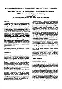
which includes: the type of the packet (“type” in Figure 2(b)), the duration of the link (“dur”), the routing path duration requirement (“EDur”), the probability of the link (“Pr”), the number of hops (“Hop”), the source and destination address (“Src”, “Dst”), the current node’s id (“ID”), the previous and next router (“pre”,“next”), the receiver of the link’s signed speed and acceleration (“rv ”,“ra ”), the sender of the link’s signed speed and acceleration (“sv ”,“sa ”), the distance of the link (“dis”). During the communication, each receiver of a link will monitor the connectivity condition of the link by computing the duration and the probability of the link. If the link is about to break, the receiver will send a control packet RBRK (Routing BReaK). The sender will send a U pd packet whose hop is set to 1. The U pd packet only explore the one-hop neighbors to find a replacement link.

In this section, we will show how the proposed scheme works. We assume that the system is composed by vehicles which install the same transceivers, GPS and with unique identities. For the purpose of this paper, we assume that the traffic is moderate in intensity, since sparse traffic renders networking as we describe it impossible. We also assumed that only the vehicles on the same direction will be recruited to propagate packets because the opposite vehicles break the routing link sooner than the same directional vehicles.

4.1

Probing the Routing Path

Due to high mobility, the topology of the network is constantly changing. Therefore, a reactive routing path probing is needed, i.e. a routing path searching is on-demand. In the literature, there are several reactive routing protocols, for example AODV, DSR, DSDV etc. which were discussed earlier. These protocols find a routing path on the basis of reachability instead of quality of the routing path. We propose a new routing path search protocol on the basis of quality of the routing path: the duration of the routing path, as well as the reachability. This is because the duration of a routing path is the most difficult and important metric to consider when routing packets in the presence of high vehicular mobility. In the routing process illustrated in Figure 2(a).a, we use the unique vehicle ID as the network address. The source vehicle will send out a probing request Prb (a control packet): PROB. Since the PROB is broadcast by wireless channel, all vehicles in the transmission range will receive it and compute the distance from the sender, the duration of the link and the probability of the link. The computation is based on the previous discussion. An acknowledgment packet AckP will be constructed by using the computed distance, duration, and probability of the link. The AckP is sent back to the sender who will collect multiple AckP and select the best link. The best link is the one with highest probability and having larger duration than the routing path duration requirement EDur. The sender only sends a confirm packet CfmP to the best link which will further explore the routing path by multicasting the Prb. When the destination node receives the probing packet, it will terminate the probing and send an acknowledgment packet back to the source node along the newly formed routing path. This completes the routing path exploration stage. The route we found is optimal in terms of long duration.

4.2

4.2.2

Global Repair

All the vehicles along the routing path know the expected expiration time of the path. These vehicles do not need to check the connectivity of the routing path if the vehicles move at constant speed. But the prediction of the routing path needs to be updated due to the dynamics of vehicular mobility where vehicles accelerate and decelerate randomly. Therefore, the connectivity of routing path needs to be updated as well. The frequency of the updating packets tupd is determined as follows. There is a fixed frequency: tuf , for example 10 seconds. Consider that there will be some short connection. Suppose ppnt is a certain percentage of the routing path duration requirement EDur. The frequency of updating packets is tuf if tuf ≤ ppnt ∗ EDur, otherwise, it is ppnt ∗ EDur if tuf > ppnt ∗ EDur. As shown in Figure 2(a).b, the source node will send a update packet U pd for every tupd seconds. When a node receives the U pd, it will compute the distance from the sender, the duration of the link and the probability of the link. The computation is based on the previous discussion and will not be repeated here. An acknowledgment packet AckU will be constructed by using the computed distance, duration, and probability of the link. The AckU is sent back to the sender who will collect multiple AckU and will select the best link which is the one with highest probability and having larger duration than the routing path duration requirement EDur. The sender only sends a confirm packet CfmU to the best link which will further explore the routing path by multicasting the U pd. When the destination node receives the update packet, it will terminate the updating process and will send an acknowledgment packet back to the source node along the latest routing path. This completes the routing path update.

Routing Path Maintenance

Usually, the route maintenance is the following: when a route is about to break, two strategies can be employed: global repair or local repair. First, the links that causes the breakage of the routing path will be locally repaired/replaced. Second, a backup route will be constructed globally before the breakage of the current routing path and will be switched as the current route. The repair procedures are based on the prediction of the link duration discussed in Section 3.1 and the probability of the link duration discussed in Section 3.2. By using this prediction, we can repair the current path before it is broken. In this way, we enhance the reliability of the routing path and maintain availability.

5.

SIMULATIONS

State of the art simulators for vehicular wireless networks involve two components: a mobility simulator and a wireless network simulator. These two components may be tightly integrated (two components in one simulator) or else loosely integrated (two components in two separated simulators but connected by trace files). In our simulator, we use looselyintegrated entities. Our mobility simulations were performed under the mobility simulation platform of Treiber and Helbing [22]. The mobility we used is IDM [23] which is close to the reality driving behaviors. We recorded the trace files of

4.2.1 Local Repair In our protocol, data packets will include a mobility header

183



vehicle mobility and then imported them into NS-2.30. In NS-2, each node represents one vehicle in the mobility simulations, moving based on the represented vehicle movement trace. Nodes in NS-2 are also entities of wireless communication nodes integrating network protocol stacks. The general parameters we used in simulations are detailed in Table 1. The total number of vehicles n is varying because in our mobility simulation, vehicles may enter and exit. The number of vehicles on the road depends on the headway distance.

rate increases because the packets have to wait if the routing links are broken, until new links are constructed. The proposed protocol gives lowest delay among the three protocols because less routing links will break. We investigated the packet delivery ratio to see how many packets were successfully delivered. As shown in Figure 4(b), both CAR and our protocol have high packet delivery ratio and our proposal even have a higher delivery ratio because of our routing path maintenance. We have also compared the throughput of the three protocols. Figure 4(c) shows the throughput comparison among the three protocols. Our protocol has higher throughput than CAR.

Table 1: The environment configure Name Value The number of vehicles (n) 1000-2000 Application CBR Network protocol IEEE 802.11 Transmission range 300m Network connections n/3 Simulation map Highway/urban Road length 5 Km Traffic density 1500 vehicles/hour Average speed 28 m/s Acceleration range [0,2] m/s2 Initial acceleration 0 m/s2 Initial speed 25 m/s Mobility model IDM [23] Car following model way-point

6.

CONCLUSION AND FUTURE WORK

In this paper we proposed a routing protocol which improves the reliability of communication in VANET. The key idea is to find a routing path with highest duration. According to the current state of mobility of vehicles, the duration of a link can be predicted by our mobility and probability model. Based on this model, the most stable links can be selected. The routing path is also updated and maintained using the mobility and probability model. Compared with the on-demand protocol DSR [24] and the mobility-based protocol ROMSGP [25], the proposed scheme has been shown effective in terms of path duration, reduced control overhead and high throughput. Additionally, compared with the probability-based routing protocol CAR [2] and the greedypropagation routing protocol GPSR [17], our protocol has been shown to feature low delay, high packet deliver ratio and high throughput. The future work includes: 1) extend the mobility model to include opposite vehicles; 2) study the communication under sparse traffic.

We simulated our routing protocol and have compared it with DSR [24] and ROMSGP [25]. DSR is a well-known ondemand routing protocol and ROMSGP is a mobility-based routing protocol. First we investigated the average duration of the routing path. The source and destination nodes are randomly selected along the vehicles on the highway. For each routing path, we recorded the path duration and obtained the average path duration. Figure 3(a) shows the average path duration for the three protocols. As it turns out, our protocol provides more stable paths than the other two protocols. This is because we select the most durable routing links. We also are interested in the control message overhead. Figure 3(a) shows the average overhead of control messages for each of the selected protocols. Compared with DSR and ROMSGP, our proposal is more efficient. For many applications, throughput is one of key factor. We compared our protocol with the other two protocols in terms of throughput. Figure 3(a) shows the average throughput of the three protocols. The throughput decreases when the speed of vehicles increases. More links will break when speed is high, thereafter, the total channels decrease and the bandwidth decreases. But, even in this scenario, our proposed protocol still outperforms both DSR and ROMSGP since fewer routing links will break under our protocol. We simulated the proposed protocol and compared it with a probability-based routing protocol CAR [2] and a wellknown greedy-propagation routing protocol GPSR [17]. Since the latter two protocols are simulated on urban map. We use SUMO [26] as our mobility simulator to record movements of all vehicles as a trace file and then, import the trace file into ns-2. To compare with the CAR and GPSR protocol, we changed our simulation parameters according to the parameters used in [2]. Figure 4(a) shows the average delay of vehicles. The delay decreases when the data

7.

REFERENCES

[1] H. Jiang, H. Guo, and L. Chen, “Reliable and efficient alarm message routing in vanet,” in ICDCSW ’08: Proceedings of the 2008 The 28th International Conference on Distributed Computing Systems Workshops. Washington, DC, USA: IEEE Computer Society, 2008, pp. 186–191. [2] Q. Yang, A. Lim, and P. Agrawal, “Connectivity aware routing in vehicular networks,” in Wireless Communications and Networking Conference, 2008. WCNC 2008. IEEE, 31 2008-April 3 2008, pp. 2218–2223. [3] G. Yan and S. Olariu, “A probabilistic analysis of path stability in vehicular ad hoc networks,” Technique Report in Computer Science of Old Dominion University, 2009. [4] G. Yan, S. Olariu, and S. El-Tawab, “Ticket-based reliable routing in vanet,” in Proceedings of the First International Workshop on Intelligent Vehicular Networks (InVeNET 2009), Macau, China, Oct 2009. [5] T. Taleb, E. Sakhaee, A. Jamalipour, K. Hashimoto, N. Kato, and Y. Nemoto, “A stable routing protocol to support its services in vanet networks,” Vehicular Technology, IEEE Transactions on, vol. 56, no. 6, pp. 3337–3347, Nov. 2007. [6] O. Abedi, M. Fathy, and J. Taghiloo, “Enhancing aodv routing protocol using mobility parameters in vanet,” in AICCSA ’08: Proceedings of the 2008

184



[7]

[8]

[9]

[10]

[11]

[12]

[13]

[14]

[15]

[16]

[17]

[18]

[19]

IEEE/ACS International Conference on Computer Systems and Applications. Washington, DC, USA: IEEE Computer Society, 2008, pp. 229–235. H. F. Wedde, S. Lehnhoff, and B. van Bonn, “Highly dynamic and scalable vanet routing for avoiding traffic congestions,” in VANET ’07: Proceedings of the fourth ACM international workshop on Vehicular ad hoc networks. New York, NY, USA: ACM, 2007, pp. 81–82. R. Morris, J. Jannotti, F. Kaashoek, J. Li, and D. Decouto, “Carnet: A scalable ad hoc wireless network system,” in In Proceedings of the 9th ACM SIGOPS European workshop: Beyond the PC: New Challenges for the Operating System. ACM Press, 2000, pp. 61–65. T. Kato, K. Kadowaki, T. Koita, and K. Sato, “Routing and address assignment using lane/position information in a vehicular ad hoc network,” in APSCC ’08: Proceedings of the 2008 IEEE Asia-Pacific Services Computing Conference. Washington, DC, USA: IEEE Computer Society, 2008, pp. 1600–1605. J. Bronsted and L. Kristensen, “Specification and performance evaluation of two zone dissemination protocols for vehicular ad-hoc networks,” in Simulation Symposium, 2006. 39th Annual, April 2006, pp. 12 pp.–. J. Gong, C.-Z. Xu, and J. Holle, “Predictive directional greedy routing in vehicular ad hoc networks,” in ICDCSW ’07: Proceedings of the 27th International Conference on Distributed Computing Systems Workshops. Washington, DC, USA: IEEE Computer Society, 2007, p. 2. M. Kihl, M. Sichitiu, T. Ekeroth, and M. Rozenberg, Reliable Geographical Multicast Routing in Vehicular Ad-Hoc Networks. Springer Berlin / Heidelberg, 2007. S. Momeni and M. Fathy, “Vanet’s communication,” in Spread Spectrum Techniques and Applications, 2008. ISSSTA ’08. IEEE 10th International Symposium on, Aug. 2008, pp. 608–612. V. Namboodiri and L. Gao, “Prediction-based routing for vehicular ad hoc networks,” Vehicular Technology, IEEE Transactions on, vol. 56, no. 4, pp. 2332–2345, July 2007. C. E. Perkins, E. M. Belding-Royer, and S. R. Das, “Ad hoc on-demand distance vector (aodv) routing,” RFC Experimental 3561, July 2003. [Online]. Available: http://rfc.net/rfc3561.txt S. Biswas, R. Tatchikou, and F. Dion, “Vehicle-to-vehicle wireless communication protocols for enhancing highway traffic safety,” Communications Magazine, IEEE, vol. 44, no. 1, pp. 74–82, Jan. 2006. B. Karp and H. T. Kung, “GPSR: greedy perimeter stateless routing for wireless networks,” in MobiCom ’00: Proceedings of the 6th annual international conference on Mobile computing and networking. New York, NY, USA: ACM, 2000, pp. 243–254. I. Greenberg, “The log-normal distribution of headways,” Australian Road Research, vol. 2, no. 7, pp. 14–18, 1966. O. C. Puan, M. R. Hainin, A. A. Chik, and Ismail, “Driver´s car following headway on single carriageway roads,” Malaysian Journal of Civil Engineering

(MJCE), vol. 16, no. 2, Jan 2004. [20] G. Yan, “Ph.d dissertation: Proving location secruity in vanet,” Computer Science Department, Old Dominion University, 2009. [21] Z. Liu, J. Almhana, and R. McGorman, “Approximating log-normal sum distributions with power log-normal distribution,” IEEE Transactions on Vehicular Technology, vol. 43, no. 4, pp. 2611–2617, July 2008. [22] “Mobility traffic simulator, http://www.mtreiber.de/index.html.” [23] M. Treiber, A. Hennecke, and D. Helbing, “Congested traffic states in empirical observations and microscopic simulations,” Physical Review E, vol. 62, p. 1805, 2000. [24] D. B. Johnson, D. A. Maltz, and Y. C. Hu, “The dynamic source routing protocol for mobile ad hoc networks (dsr),” Published Online, IETF MANET Working Group, Tech. Rep., February 2007. [25] T. Taleb, E. Sakhaee, A. Jamalipour, K. Hashimoto, N. Kato, and Y. Nemoto, “A stable routing protocol to support its services in vanet networks,” Vehicular Technology, IEEE Transactions on, vol. 56, no. 6, pp. 3337–3347, Nov. 2007. [26] Open source, “Simulation of urban mobility,” http://sumo.sourceforge.net.

APPENDIX A. LINK DURATION CASES Due to the page limit, we list link duration case a. For more detailed discussion or the rest of cases, refer our previous research [20]. In Case a, only tβ and tε exist, as shown in figure 1.a. We can obtain the link duration time t. Let {ai > 0 > aj ; vj > vi > 0} be condition one, marked as c1 ; {aj > 0 > ai ; vi > vj > 0} be condition two, marked as c2 . √ 2  −vr + vr +2ar (300−X)   , {c1 ; 0 ≤ t ≤ tα }  √ 2 ar    v −2a (300+X) −v − r r r   , {c1 ; tα < t ≤ tε }  ar q    2 −2a (300+X+ vm −vi t ) −(v −v )− (v −v )  m m ε j j j 2  , {c1 ; tε < t < tβ }  aj   vj  vm −vi   300+x+ 2 tε + 2 tβ , {c1 ; tβ < t} √ 2 vm t= −vr − vr −2ar (300+X)   , {c2 ; 0 ≤ t ≤ tα }   √ 2 ar   −vr + vr +2ar (300−X)   , {c2 ; tα < t ≤ tε }  arq    −(vj −vm )− (vj −vm )2 −2ai (300−X+ vm −vi tε )  2   , {c2 ; tε < t ≤ tβ }  aj   vm −vj vi   300−X+ 2 tε − 2 tβ , {c2 ; tβ < t} vm

185

Proceedings of MoMM2009 m

j

i


i

j

j

i

i

j

i

j

i

i

j

i

j

j

β

m

i

j

i

i

j

j

i

j

i

i

j

j

i i

(d)

(c)

(b)

m

β

β

β

(a)

j

m

m

m

j β

(f)

(e)

γ

α

γ

β

(g)

(h)

Figure 1: Illustrating the same direction case.

Receiver Prb

Sender

Sender

AckP

Receiver Upd

type

dur

EDur

Pr

hop

Src

Dst

ID

pre

next

r_v

r_a

s_v

s_a

dis

AckU

CfmP

CfmU

Others (len, chksum, priority, sig, etc)

(b)

(a) (a)

(b)

The proposed protocol

The packet header

Figure 2: The protocol and packet header 1000

Average path duration (s)

DSR ROMSGP The proposed 150

100

50

0

0

5

10

15

20

25

30

DSR ROMSGP The proposed

5

4

600

3

400

2

200

1

35

0

5

10

The speed (m/s)

(a)

DSR ROMSGP The proposed

800

Average path duration (s)

Control overhead (# of control packets) [10^6]

200

15

20

25

30

0

35

0

5

10

15

The speed (m/s)

(b)

Duration

20

25

30

The speed (m/s)

(c)

Control message overhead.

Throughput

Figure 3: Comparison with mobility-based routing

1

25

150 0.8

15

CAR GPRS The proposed

Throughput (kb/s)


Delivery ratio

Delay (sec)

20

0.6

10

0.4

5

0.2

100

50

0

0.2

0.4

0.6

Data sending rate (kb/s)

(a)

Delay.

0.8

1


0

0.2

0.4

0.6

0.8

1

0

0

200


(b)

Delivery ratio.

Figure 4: Comparison with probability-based routing

186

400

600

800


(c)

Throughput.

1000

35