Hawthorn, Melbourne, Australia 3122 ...... deployed at all primary hosting nodes as exemplified in the top of plane of Figure 7 .... and Web Service Processes.
A Probabilistic Strategy for Setting Temporal Constraints in Scientific Workflows Xiao Liu, Jinjun Chen, and Yun Yang Faculty of Information and Communication Technologies Swinburne University of Technology Hawthorn, Melbourne, Australia 3122 {xliu,yyang,jchen}@swin.edu.au
Abstract. In scientific workflow systems, temporal consistency is critical to ensure the timely completion of workflow instances. To monitor and guarantee the correctness of temporal consistency, temporal constraints are often set and then verified. However, most current work adopts user specified temporal constraints without considering system performance, and hence may result in frequent temporal violations that deteriorate the overall workflow execution effectiveness. In this paper, with a systematic analysis of such problem, we propose a probabilistic strategy which is capable of setting coarse-grained and finegrained temporal constraints based on the weighted joint distribution of activity durations. The strategy aims to effectively assign a set of temporal constraints which are well balanced between user requirements and system performance. The effectiveness of our work is demonstrated by an example scientific workflow in our scientific workflow system. Keywords: Scientific Workflow, Temporal Constraints, Temporal Constraint Setting, Probabilistic Strategy.
1 Introduction Scientific workflow is a new special type of workflow that often underlies many large-scale complex e-science applications such as climate modelling, structural biology and chemistry, medical surgery or disaster recovery simulation [18][25]. Real world scientific as well as business processes normally stay in a temporal context and are often time constrained to achieve on-time fulfilment of certain scientific or business targets. Furthermore, scientific workflows are usually deployed on the high performance computing infrastructures, e.g. cluster, peer-to-peer and grid computing, to deal with huge number of data intensive and computation intensive activities [24][25]. Therefore, as an important dimension of workflow QoS (Quality of Service) constraints, temporal constraints are often set to ensure satisfactory efficiency of scientific workflow executions [5][9]. Temporal constraints mainly include three types, i.e. upper bound, lower bound and fixed-time. An upper bound constraint between two activities is a relative time value so that the duration between them must be less than or equal to it. As discussed in [6], conceptually, a lower bound constraint is symmetrical to an upper bound constraint and a fixed-time constraint can be viewed as a M. Dumas, M. Reichert, and M.-C. Shan (Eds.): BPM 2008, LNCS 5240, pp. 180–195, 2008. © Springer-Verlag Berlin Heidelberg 2008
A Probabilistic Strategy for Setting Temporal Constraints in Scientific Workflows
181
special case of upper bound constraint, hence they can be treated similarly. Therefore, in this paper, we focus on upper bound constraints only. As an important means to facilitate temporal QoS, many efforts have been dedicated to temporal verification for workflows in recent years. Different approaches for checkpoint selection and dynamic temporal verification are proposed to improve the efficiency of temporal verification with given temporal constraints [6][10][17]. However, with the assumption that temporal constraints are pre-defined, most papers focus on run-time temporal verification while neglecting the fact that efforts put at run-time will be mostly in vain without build-time setting of high quality temporal constraints. The reason is obvious since the purpose of temporal verification is to identify potential violations of temporal constraints to minimise the exception handling cost. Therefore, if temporal constraints are of low quality themselves, temporal violations are highly expected no matter how much efforts have been put by temporal verification. The task of setting temporal constraints described in this paper is to assign a set of coarse-grained and fine-grained upper bound temporal constraints to scientific workflows. Here, coarse-grained constraints refer to those assigned to the entire workflow or workflow segments, while fine-grained constraints refer to those assigned to individual activities. However, although coarse-grained constraints can be deemed as the collection of fine-grained constraints, they are not in a simple relationship of linear culmination and decomposition. To ensure on-time fulfilment of workflow instances, both coarse-grained and fine-grained temporal constraints are required, especially when scientific workflows are deployed on dynamic computing infrastructures, e.g. grid, where the performance of the underlying resources is highly uncertain [18]. Here, the quality of temporal constraints can be measured by at least two criteria: 1) well balanced between user requirements and system performance; 2) well supported for both overall coarse-grained control and local fine-grained control. A detailed illustration will be presented in Section 2. In this paper, a probabilistic strategy for setting both coarse-grained and finegrained temporal constraints is proposed. With a novel probability based temporal consistency which utilises the weighted joint distribution of activity durations, our strategy supports an iterative and interactive negotiation process between the client (e.g. a user) and the service provider (e.g. a workflow system) for setting coarsegrained temporal constraints. Afterwards, fine-grained temporal constraints associated with each activity can be derived automatically. In addition, the weighted joint distribution of four basic Stochastic Petri Nets [1] (SPN) based building blocks, i.e. sequence, iteration, parallelism and choice, is presented to enhance the efficiency of calculating the overall weighted joint distribution through their compositions. The effectiveness of our strategy is further demonstrated by an example scientific workflow of weather forecast in our scientific workflow management system, i.e. SwinDeW-G (Swinburne Decentralised Workflow for Grid) [23]. The remainder of the paper is organised as follows. Section 2 presents a motivating example and the problem analysis. Section 3 proposes novel probability based temporal consistency. Section 4 presents the probabilistic strategy for setting temporal constraints. Section 5 further demonstrates the setting process with the motivating example to verify the effectiveness of our strategy. Section 6 introduces the implementation of the strategy in our scientific workflow system. Section 7 presents the related work. Finally, Section 8 addresses our conclusion and future work.
182
X. Liu, J. Chen, and Y. Yang
2 Motivating Example and Problem Analysis In this section, we introduce a weather forecast scientific workflow to demonstrate the problem of setting temporal constraints. In addition, two basic requirements for setting high quality temporal constraints are presented. The entire weather forecast workflow contains hundreds of data intensive and computation intensive activities. Major data intensive activities include the collection of meteorological information, e.g. surface data, atmospheric humidity, temperature, cloud area and wind speed from satellites, radars and ground observatories at distributed geographic locations. These data files are transferred via various kinds of network. Computation intensive activities mainly consist of solving complex meteorological equations, e.g. meteorological dynamics equations, thermodynamic equations, pressure equations, turbulent kinetic energy equations and so forth which require high performance computing resources. Due to the space limit, it is not possible to present the whole forecasting process in detail. Here, we only focus on one of its segments for radar data collection. As depicted in Figure 1, this workflow segment contains 12 activities which are modeled by SPN with additional graphic notations as illustrated in Sections 4 and 6. For simplicity, we denote these activities as X 1 to X 12 . The workflow process structures are composed with four SPN based building blocks, i.e. a choice block for data collection from two radars at different locations (activities X 1 ~ X 4 ), a compound block of parallelism and iteration for data updating and pre-processing (activities X 6 ~ X 10 ), and two sequence blocks for data transferring (activities X 5 , X 11 , X 12 ). It is evident that the duration of these scientific workflow activities are highly dynamic in nature due to their data complexity and the computation environment. However, to ensure the weather forecast can be broadcast on time, every scientific workflow instances must be completed within a specific time duration. Therefore, a set of temporal constraints must be set to monitor the overall workflow execution time. For our example workflow segment, to ensure that the radar data can be collected in time and transferred for further processing, at least one overall upper bound temporal constraint is required. However, a coarse-grained temporal constraint is not effective enough to ensure fine-grained workflow execution, i.e. the completion time of each activity. It is evidently that without the support of local enforcements, the overall workflow duration can hardly be guaranteed. For example, we set a two hour temporal constraint for this radar data collection process. But due to some technical problems, the connection to the two radars are broken and blocked in a state of retry
Fig. 1. Example scientific workflow segment
A Probabilistic Strategy for Setting Temporal Constraints in Scientific Workflows
183
and timeout for more than 30 minutes whilst its normal duration should be far less. Therefore, the two hour overall temporal constraint for this workflow segment will probably be violated since its subsequent activities normally require more than 90 minutes to accomplish. However, no actions were taken yet due to the ignorance of the fine-grained temporal constraints on these connection activities. The exception handling cost for compensation of this time deficit, e.g. workflow re-scheduling and recruitment of additional resources, is hence inevitable. That is why we also need to set fine-grained temporal constraints to each activity. Specifically, for this example workflow segment, an overall coarse-grained temporal constraint and 12 fine-grained temporal constraints for activities X 1 to X 12 are required to be set. However, setting temporal constraints is not a straightforward task, many factors such as workflow structures, system performance and user requirements should be taken into consideration. Here, we present the basic requirements of the setting strategy by analysing two criteria for high quality temporal constraints. 1) Temporal constraints should be well balanced between user requirements and system performance. It is common that clients often suggest coarse-grained temporal constraints based on their own interest while with limited knowledge about the actual performance of workflow systems. With our example, it is not rational to set a 60 minutes temporal constraint to the segment which normally needs two hours to finish. Therefore, user specified constraints are normally prone to cause frequent temporal violations. To address this problem, a negotiation process between the client and the service provider who is well aware of the system performance is desirable to achieve balanced coarse-grained temporal constraints that both sides are satisfied with. 2) Temporal constraints should facilitate both overall coarse-grained control and local fine-grained control. As analysed above, this criterion actually means that the strategy should support setting both coarse-grained temporal constraints and finegrained temporal constraints. However, although the overall workflow process is composed of individual workflow activities, coarse-grained temporal constraints and fine-grained temporal constraints are not in a simple relationship of linear culmination and decomposition. Meanwhile, it is impractical to set fine-grained temporal constraints manually for a large amount of activities in scientific workflows. Since coarse-grained temporal constraints can be obtained through the negotiation process, the problem to be addressed here is how to automatically derive the local fine-grained temporal constraints for each activity. To conclude, the basic requirements for setting high quality temporal constraints can be simply put as effective negotiation for coarse-grained temporal constraints and automatic assignment for fine-grained temporal constraints. However, to our best knowledge, very little efforts have been dedicated to set high quality temporal constraints in scientific workflows. In this paper, we propose a probabilistic strategy which targets at the two requirements.
3 Probability Based Temporal Consistency In this section, we propose a novel probability based temporal consistency which utilise the weighted joint distribution of workflow acitivity durations to facilitate setting temporal constraints. To define the weighted joint distribution of workflow
184
X. Liu, J. Chen, and Y. Yang
acitivity durations, we first present two assumptions on the probability distribution of individual activity duration. Assumption 1: The distribution of activity durations can be obtained from workflow system logs. Without losing generality, we assume all the activity durations follow the normal distribution model, which can be denoted as N ( μ , σ 2 ) where μ is the expected value and σ 2 is the variance where σ is the standard deviation [21]. Assumption 2: The activity durations are independent to each other. For the convenience of analysis, assumption 1 chooses normal distribution to model the activity durations. If most of the activity durations follow non-normal distribution, e.g. Gamma distribution, lognormal distribution or Beta distribution [16], our strategy can still be applied in a similar way with minor differences of their joint distribution. Furthermore, as it is commonly applied in the area of system simulation and performance analysis, assumption 2 requires that the activity durations be independent from each other to facilitate the analysis of joint normal distribution. For those which do not follow the above assumptions, they can be treated by normal transformation and correlation analysis [16], or moreover, they can be ignored first when calculating joint distribution and then added up afterwards. Furthermore, we present an important formula of joint normal distribution. Formula 1: If there are n independent variables of X i ~ N ( μ i , σ i2 ) and n real num-
bers θ i , where n is a limited natural number, then the joint distribution of these variables can be obtained with the following formula [21]: n n ~ N ⎛⎜ ∑ θ i μ i , ∑ θ i2σ i2 ⎞⎟ (1) i =1 ⎝ i =1 ⎠ Based on this formula, we define the weighted joint distribution of workflow acitivity durations as follows. Definition 1: (Weighted joint distribution). For a scientific workflow process SW which consists of n activities, we denote the activity duration distribution of
Z = θ 1 X 1 + θ 2 X 2 + ... + θ n X n =
n ∑θi X i i =1
activity a i as N ( μ i , σ i2 ) with 1 ≤ i ≤ n . Then the weighted joint distribution is defined n ⎛n ⎞ 2 as N ( μ sw , σ sw ) = N ⎜ ∑ wi μ i , ∑ wi2σ i2 ⎟ , where wi stands for the weight of activity i =1 ⎠ ⎝ i =1 ai that denotes the choice probability or iteration times associated with the workflow path where ai belongs to.
The weight of each activity with different kinds of workflow structures will be further illustrated in Section 4 by the calculation of weighted joint distribution for basic SPN based building blocks. The weighted joint distribution enables us to analyse the completion time of the entire workflow from an overall perspective. Here, we need to define some notations. For a workflow activity ai , its maximum duration and minimum duration are defined as D(ai ) and d (a i ) respectively. For a scientific workflow process SW which consists of n activities, its upper bound temporal constraint is denoted as U (SW ) with the value of u (SW ) [6][10]. In addition, we employ the “ 3σ ”rule which has been widely used in statistical data analysis to specify the
A Probabilistic Strategy for Setting Temporal Constraints in Scientific Workflows
185
possible intervals of activity durations. The “ 3σ ”rule depicts that for any sample comes from normal distribution model, it has a probability of 99.73% to fall into the range of [μ − 3σ , μ + 3σ ] which is a systematic interval of 3 standard deviation around the mean [21]. Therefore, in this paper, we define the maximum duration as D(a i ) = μ i + 3σ i and the minimum duration as d (a i ) = μ i − 3σ i . Accordingly, samples from the system logs which are above D(ai ) or below d (a i ) are hence discarded as outliers. Now, we propose the definition of probability based temporal consistency which is based on the weighted joint distribution of activity durations. To be noted that, since we deal with setting temporal constraints in this paper, here we only present the definition of build-time temporal consistency. Definition 2: (Probability based temporal consistency). At build-time stage, U (SW ) is said to be: n ∑ wi ( μ i + 3σ i ) ≤ u ( SW ) ; i =1 n Absolute Inconsistency (AI), if ∑ wi ( μ i − 3σ i ) ≥ u ( SW ) ; i =1 n α % Consistency ( α % C), if ∑ wi ( μ i + λσ i ) = u ( SW ) . i =1
1) Absolute Consistency (AC), if 2) 3)
Here wi stands for the weight of activity ai , λ ( −3 ≤ λ ≤ 3 ) is defined as the α % confidence percentile with the cumulative normal distribution function of F ( μ i + λσ i ) =
1
σ 2π
μi + λσ i ∫− ∞
h
− ( x − μi ) 2
2σ i2
• dx = α % ( 0 < α < 100 ). As depicted in
Figure 2, if we apply the “ 3σ ”rule to the conventional discrete multiple temporal consistency [7], i.e. strong consistency (SC), weak consistency (WC), weak inconsistency (WI) and strong inconsistency (SI), the two discrete states of WI and WC are actually replaced by continuous consistency states α % C which compose a Gaussian curve the same as the cumulative normal distribution [21]. The other two consistency states outside the interval are basically the same but also with continuous values infinitely approaching 100% or 0% respectively. However, in order to distinguish them from conventional strong consistency and strong inconsistency, we name them absolute consistency (AC) and absolute inconsistency (AI). Evidently, the prerequisite for this definition is the calculation of weighted joint distribution.
Fig. 2. Probability based temporal consistency
186
X. Liu, J. Chen, and Y. Yang
The purpose of probability based temporal consistency is to facilitate the effectiveness of setting temporal constraints. The reason why conventional discrete multiple states based temporal consistency is not suitable here can be explained from two aspects. First, clients normally cannot distinguish between qualitative expressions such as weak consistency and weak inconsistency due to the lack of background knowledge, and thus deteriorates the negotiation process for setting coarse-grained temporal constraints. Second, since each discrete temporal consistency state is actually defined with a coarse-grained interval, it cannot support fine-grained setting. Hence, we propose the probability based continuous temporal consistency. A probability value such as 80% or 90% gives much more sense than a qualitative expression, and any finegrained temporal consistency state is represented by a unique probability value rather than the previous coarse-grained qualitative expression for each interval. Therefore, the probability based temporal consistency supports the setting of both coarse-grained and fine-grained temporal constraints.
4 Probabilistic Strategy for Setting Temporal Constraints In this section, we present our probabilistic strategy for setting temporal constraints. The strategy aims to effectively achieve a set of coarse-grained and fine-grained temporal constraints which are well balanced between user requirements and system performance. As depicted in Table 1, the strategy requires the input of process model and system logs. It consists of three steps, i.e. calculating weighted joint distribution of activity durations, setting coarse-grained temporal constraints and setting fine-grained temporal constraints. We illustrate them accordingly as follows. The first step is to calculate weighted joint distribution. The statistic information, i.e. activity duration distribution and activity weight, can be obtained from system logs by statistical analysis [1][21]. Here, to illustrate and facilitate the calculation of the weighted joint distribution, we analyse basic SPN based building blocks, Table 1. Probabilpistic setting strategy
A Probabilistic Strategy for Setting Temporal Constraints in Scientific Workflows
187
i.e. sequence, iteration, parallelism and choice. These four building blocks consist of basic control flow patterns and are widely used in workflow modelling and structure analysis [2][4][19]. Most workflow process models can be easily built by their compositions, and similarly for the weighted joint distribution of most workflow processes. Here, SPN based modelling is employed to incorporate time and probability stands for the probability of the attributes with additional graphic notations, e.g. path and stands for the normal duration distribution of the associated activity. For simplicity, we consider two paths for the iteration, parallelism and choice building blocks, except the sequence building block which has only one path by nature. However, the results can be extended to more paths in a similar way. 1) Sequence building block. As depicted in Figure 3, the sequence building block is composed by adjacent activities from ai to a j in a sequential relationship which
means the successor activity will not be executed until its predecessor activity is finished. The weight for each activity in the sequence building block is 1 since they only need to be executed once. Therefore, according to Formula 1, the weighted joint disj j ⎛ j ⎞ tribution is Z = ∑ X k ~ N ⎜ ( ∑ μ k ), ( ∑ σ k2 ) ⎟ . k =i k =i ⎝ k =i ⎠ 2) Iteration building block. As depicted in Figure 4, the iteration building block contains two paths which are executed iteratively until certain end conditions are satisfied. If the probability of meeting the end conditions for a single iteration is γ as denoted by the probability notation, then the lower path is expected to be executed for 1 r times and hence the upper path is executed for (1 r ) + 1 times. Accordingly, the weight for each activity in the iteration building block is the expected execution times of the path it belongs to. Therefore, the weighted joint distribution here is j j l l ⎛j ⎞ ⎛ l ⎞ ⎛⎛ ⎞⎛ ⎞⎞ Z =((1γ) +1)⎜⎜ ∑ Xp⎟⎟+(1γ)⎜⎜ ∑ Xq⎟⎟ ~ N⎜⎜⎜((1γ) +1)( ∑ μp) +(1γ)( ∑ μq)⎟⎟,⎜⎜((1γ) +1)2( ∑ σ2p) +(1γ)2( ∑ σq2)⎟⎟⎟ . ⎜ p=i q=k ⎠⎟⎠ p=i q=k ⎠ ⎝ ⎝p=i ⎠ ⎝q=k ⎠ ⎝⎝ 3) Parallelism building block. As depicted in Figure 5, the parallelism building block contains two paths which are executed in a parallel relationship. The overall completion time of the parallelism building block is dominated by the path with the longer duration. Hence the joint distribution of this building block equals the joint j
l
p =i
q=k
distribution of the path with a lager expected total duration, that is if ∑ μ p ≥ ∑ μ q then Z =
j ∑ μp p =i
, otherwise Z =
l ∑ q=k
μ q . Evidently, the weight for each activity on the
Fig. 3. Sequence building block
188
X. Liu, J. Chen, and Y. Yang
Fig. 4. Iteration building block
path with longer duration is 1 while on the other path is 0 since they do not contribute to the joint distribution. Therefore, the weighted joint distribution of this block j ⎛ j ⎧ j 2 ⎞⎟ ⎜ ⎪⎪ ∑ X p ~ N ⎜ p∑=i μ p , p∑=i σ p ⎟ , if ∑j μ ≥ ∑l μ ⎝ ⎠ p q . is Z = ⎨ pl=i p =i q=k l l ⎛ ⎞ , 2 ⎪ ∑ X q ~ N⎜ ∑ μ , ∑ σ ⎟ otherwise ⎜ q =k q q =k q ⎟ ⎪⎩q = k ⎝ ⎠
Fig. 5. Parallelism building block
4) Choice building block. As depicted in Figure 6, the choice building block contains two paths in an exclusive relationship which means only one path will be executed at run-time. The probability notation denotes that the probability for the choice of the upper path is β and hence the probability for the lower path is 1 − β . The weight for each activity in the choice building block is hence the probability of the path it belongs to. Therefore, the weighted joint distribution j j l l l ⎛ j ⎞ is Z = β ( ∑ X p ) + (1− β )( ∑ X q ) ~ N⎜⎜β( ∑ μp ) +(1−β)( ∑ μq ),β 2( ∑ σ 2p ) +(1−β)2( ∑ σq2)⎟⎟ . p=i q=k q=k p=i q=k ⎝ p=i ⎠ The second step is to set coarse-grained temporal constraints. Based on the four basic building blocks, the weighted joint distribution of an entire workflow or workflow segment can be obtained efficiently to facilitate the negotiation process for setting coarse-grained temporal constraints. Here, we denote the obtained weighted joint distribution of the target scientific workflow (or workflow segment) SW 2 as N ( μ sw , σ sw ) and assume the minimum threshold is β % for the probability consistency which implies client’s acceptable bottom-line probability for timely completion of the workflow instance. The actual negotiation process starts with the client’s initial suggestion of an upper bound temporal constraint of u (SW ) and the evaluation of the corresponding temporal consistency state by the service provider. If u ( SW ) = μ sw + λσ sw with λ as the α % percentile, and α % is below the threshold
A Probabilistic Strategy for Setting Temporal Constraints in Scientific Workflows
189
Fig. 6. Choice building block
of β % , then the upper bound temporal constraint needs to be adjusted, otherwise the negotiation process terminates. The subsequent process is the iteration that the client proposes new upper bound temporal constraint which is less constrained as the previous one and the service provider re-evaluates the consistency states, until it reaches or is above the minimum probability threshold. The third step is to set fine-grained temporal constraints. In fact, this process is straight forward with the probability based temporal consistency. Since our temporal consistency actually defines that if all the activities are executed with the duration of α % probability and their total weighted duration equals their upper bound constraint, we say that the workflow process is α % consistency at build-time. For example, if the obtained probability consistency is 90% with the percentile λ of 1.28 (the percentile value can be obtained from any normal distribution table or most statistic program [21]), it means that all activities are expected for the duration of 90% probability. Therefore, after the achievement of the coarse-grained temporal constraint, the finegrained temporal constraint for activity ai with N ( μ i , σ i2 ) is as μ i + λσ i automatically. In the case of 90% consistency, it is μ i + 1.28σ i .
derived
5 Evaluation In this section, we evaluate the effectiveness of our strategy by further illustrating the motivating example introduced in Section 2. The process model is the same as depicted in Figure 1. As presented in Table 1, the first step is to calculate the weighted joint distribution. Based on statistical analysis and the “ 3σ ”rule, the normal distribution model and its associated weight for each activity duration are specified through statistical analysis of accumulated system logs. Therefore, as depicted in Table 2, the weighted joint distribution of each building block can be derived instantly with their formulas proposed in Section 4. We obtain the weighted joint distribution for the workflow segment as N (6210,218 2 ) with second as the basic time unit. The detailed specification of the workflow segment is presented in Table 2. The second step is the negotiation process for setting an overall upper bound temporal constraint for this workflow segment. Here, we assume that the client’s expected minimum threshold of the probability consistency state be 80%. The client starts to propose an upper bound temporal constraint of 6300s, based on the weighted joint distribution of N (6210,218 2 ) and the cumulative normal distribution function, the service provider can obtain the percentile as λ = 0.41 and reply with the probability of 66% which is lower than the threshold. Hence the service provider advises the
190
X. Liu, J. Chen, and Y. Yang Table 2. Specification of the workflow segment
client to relax the temporal constraint. Afterwards, for example, the client proposes a series of new candidate upper bound temporal constraints one after another, e.g. 6360s, 6390s and 6400s, and the service provider replies with 75%, 79% and 81% as the corresponding temporal consistency states. Therefore, through this negotiation process, the final negotiation result could be an upper bound temporal constraint of 6400s with a probability consistency state of 81%. The third step is to set the fine-grained constrains for each workflow activity with the obtained overall upper bound constraint. As we mentioned in Section 4, the probability based temporal consistency defines that the probability for each expected activity duration is the same as the probability consistency state of the workflow process. Therefore, since the coarse-grained temporal constraint is 6400s with a probability consistency state of 81%, the probability of each activity duration is also 81%. According to the normal distribution, 81% means a percentile of λ = 0.87 . Hence, the fine-grained temporal constraints for each activity can be calculated by μ + 0.87σ . For example, the fine-grained upper bound temporal constraint for activity X 1 is (105 + 0.87 * 225 ) = 118s and the upper bound constraint for activity X 12 is (123 + 0.87 * 64 ) = 130s . The detailed results are presented in Table 3. Table 3. The setting results
A Probabilistic Strategy for Setting Temporal Constraints in Scientific Workflows
191
To conclude, the above demonstration of the setting process evidently shows that our probabilistic strategy is effective for setting both coarse-grained and fine-grained temporal constraints. Meanwhile, it has met the two basic requirements proposed in Section 2, i.e. effective negotiation and automatic setting.
6 System Implementation In this section, we introduce the implementation of the setting strategy in our SwinDew-G scientific grid workflow system. 6.1 SwinDeW-G Scientific Workflow System
SwinDeW-G is a peer-to-peer based scientific grid workflow system running on the SwinGrid (Swinburne service Grid) platform [23]. An overall picture of SwinGrid is depicted in Figure 7 (bottom plane) which contains many grid nodes distributed in different places. Each grid node contains many computers including high performance PCs and/or supercomputers composed of significant number of computing units. The primary hosting nodes include the Swinburne CITR (Centre for Information Technology Research) Node, Swinburne ESR (Enterprise Systems Research laboratory) Node, Swinburne Astrophysics Supercomputer Node, and Beihang CROWN (China R&D environment Over Wide-area Network) Node in China. They are running Linux, GT4 (Globus Toolkit) or CROWN grid toolkit 2.5 where CROWN is an extension of GT4 with more middleware, hence compatible with GT4. Currently, SwinDeW-G is deployed at all primary hosting nodes as exemplified in the top of plane of Figure 7 (top plane). In SwinDeW-G, a scientific workflow is executed by different peers that may be distributed at different grid nodes. As shown in Figure 6, each grid node can have a number of peers, and each peer can be simply viewed as a grid service. As an important reinforcement for the overall workflow QoS, temporal verification is being implemented in SwinDeW-G. It currently supports dynamic checkpoint selection and temporal verification at run-time [9]. After the running of SwinDeW-G for a period of time, statistical analysis can be applied to accumulated system logs to obtain probability attributes. The probabilistic strategy for setting temporal constraints is being integrated into the scientific workflow modelling tool which supports SPN based modelling, composition of building blocks, temporal data analysis, interactive and automatic setting of temporal constraints. 6.2 SwinDeW-G Scientific Workflow Modelling Tool
Our probabilistic strategy for setting temporal constraints is being implemented into our SwinDeW-G scientific workflow system as an integrated component of the modelling tool. As shown in Figure 8(a), the modelling tool adopts SPN with additional graphic notations, e.g. for probability, for activity duration, for a subfor the start point and for the end point of an upper bound temporal process, constraint, to support explicit representation of temporal information. It also supports the composition of the four basic building blocks and user specified ones. The component supports temporal data analysis from workflow system logs. Temporal data
192
X. Liu, J. Chen, and Y. Yang
Fig. 7. Overview of SwinDeW-G environment
analysis follows the “ 3σ ”rule and can generate the normal distribution model for each activity duration. The probability attributes for each workflow structure such as the choice probability and iteration times can also be obtained through statistical analysis on historic workflow instances from system logs. After temporal data analysis, the attributes for each activity, i.e. its mean duration, variance, maximum duration, minimum duration and weight are associated to the corresponding activity and explicitly displayed to the client. Meanwhile, the weighted joint distribution of the target process is obtained automatically with basic building blocks. As shown in Figure 8(b), with our probability based temporal consistency, the client can specify an upper bound temporal constraint and the system will reply with a probability for the consistency state. Based on the visualised results shown by a Gaussian curve (the cumulative normal distribution), the client can decide whether to accept or decline the results. If the client is not satisfied with the outcomes, he or she can specify a new value for evaluation until a satisfactory result is achieved. Evidently, the negotiation process between the client and the service provider is implemented as an interactive
(a) Temporal data analysis
(b) Setting temporal constraints
Fig. 8. SwinDeW-G modelling tool
A Probabilistic Strategy for Setting Temporal Constraints in Scientific Workflows
193
process between the system user and our developed program. After setting the coarsegrained temporal constraints, the fine-grained constraints for each activity areassigned automatically. These activity duration distribution models, coarse-grained and finegrained temporal constraints are explicitly represented in the scientific workflow models and will be further deployed to facilitate the effectiveness of run-time temporal verification in scientific workflows.
7 Related Work In this section, we review some related work on temporal constraints in both traditional workflows and non-traditional workflows. The work in [24] presents the taxonomy of grid workflow QoS constraints which include five dimensions, i.e. time, cost, fidelity, reliability and security. Some papers have presented an overview analysis of scientific or grid workflow QoS [5][14]. The work in [8] presents the taxonomy of grid workflow verification which includes the verification of temporal constraints. Generally speaking, there are two basic ways to assign QoS constraints, one is tasklevel assignment and the other is workflow-level assignment. Since the whole workflow process is composed by all individual tasks, an overall workflow-level constraint can be obtained by the composition of task-level constraints. On the contrary, tasklevel constraints can also be assigned by the decomposition of workflow-level constraints [24]. However, different QoS constraints have their own characteristics and require in depth research to handle different scenario. As shown in our setting strategy, the primary information required for setting temporal constraints include the workflow process models, statistics for activity durations and the definition of temporal consistency. Scientific workflows require the explicit representation of temporal information, i.e. activity durations and temporal constraints to facilitate temporal verification. One of the classical modelling methods is the Stochastic Petri Net (SPN) [1][4] which incorporates time and probability attributes into workflow processes that can be employed to facilitate scientific workflow modelling. Activity duration, as one of the basic elements to measure system performance, is of significant value to workflow scheduling, performance analysis and temporal verification [8][18]. Most work obtains activity durations from workflow system logs and describes them by a discrete or continuous probability distribution through statistical analysis [1]. As for temporal consistency, traditionally, there are only binary states of consistency or inconsistency. However, as stated in [7], it argues that the conventional consistency condition is too restrictive and covers several different states which should be handled differently for the purpose of cost saving. Therefore, it divides conventional inconsistency into weak consistency, weak inconsistency and strong inconsistency and treats them accordingly. However, as we discussed in Section 3, multiple discrete temporal consistency is not quite effective in terms of negotiation and setting for temporal constraints. Temporal constraints are not well emphasised in traditional workflow systems. However, some business workflow systems accommodate temporal information for the purpose of performance analysis. For example, Staffware provides the audit trail tool to monitor the execution of individual instances [2] and SAP business workflow system employs the workload analysis [22]. As for scientific workflow systems, according to the survey conducted in [24], Askalon [3], GrADS [11], GridBus [12] and
194
X. Liu, J. Chen, and Y. Yang
GridFlow [13] support temporal constraints and some other QoS constraints. Yet, to our best knowledge, only SwinDeW-G [23] has set up a series of strategies such as multiple temporal consistency states and efficient checkpoint selection to support dynamic temporal verification [7][9]. In overall terms, even though temporal QoS has been recognised as an important aspect in scientific workflow systems, the work in this area, e.g. the specification of temporal constraints and the support of temporal verification, is still in its infancy.
8 Conclusion and Future Work In this paper, we have proposed a probabilistic strategy for setting temporal constraints in scientific workflows. The strategy aims to achieve a set of temporal constraints which are well balanced between user requirements and system performance. Hence, novel probability based temporal consistency which is defined by the weighted joint distribution of activity durations has been provided to support an effective negotiation process between the client and the service provider. In addition, the weighted joint distribution of four Stochastic Petri Nets based basic building blocks, i.e. sequence, iteration, parallelism and choice, has been presented to facilitate the setting process. With the probability based temporal consistency, well balanced overall coarse-grained temporal constraints can be achieved through the negotiation process, and afterwards, fine-grained temporal constraints for each activity can be derived instantly in an automatic fashion. A weather forecast scientific workflow has been first employed as a motivating example and then revisited with the detailed setting process to evaluate the effectiveness of our strategy. As an integrated component of the scientific workflow modelling tool in our SwinDeW-G scientific grid workflow system, the probabilistic strategy has been effectively implemented to support the setting of both coarse-grained and fine-grained temporal constraints in scientific workflows. In the future, with our probability based temporal consistency, we will investigate corresponding run-time strategies for checkpoint selection, temporal verification and temporal-constraint adjustment, so as to improve the overall efficiency and effectiveness of temporal verification in scientific workflows. Acknowledgments. The research work reported in this paper is partly supported by Australian Research Council under Discovery Grant DP0663841, Linkage Grant LP0669660, by Swinburne Dean’s Collaborative Grants Scheme 2007-2008, and by Swinburne Research Development Scheme 2008.
References 1. van der Aalst, W.M.P., Hee, K.M.V., Reijers, H.A.: Analysis of Discrete-Time Stochastic Petri Nets. Statistica Neerlandica 54, 237–255 (2000) 2. van der Aalst, W.M.P., Hee, K.M.V.: Workflow Management: Models, Methods, and Systems. The MIT Press, Cambridge (2002) 3. Askalon Project (accessed March 1, 2008), http://www.dps.uibk.ac.at/projects/askalon 4. Bucci, G., Sassoli, L., Vicario, E.: Correctness Verification and Performance Analysis of Real-Time Systems Using Stochastic Preemptive Time Petri Nets. IEEE Trans. on Software Engineering 31(11), 913–927 (2005)
A Probabilistic Strategy for Setting Temporal Constraints in Scientific Workflows
195
5. Cardoso, J., Sheth, A., Miller, J., Arnold, J., Kochut, K.: Quality of Service for Workflows and Web Service Processes. Journal of Web Semantics: Science, Service and Agents on the World Wide Web 1(3), 281–308 (2004) 6. Chen, J., Yang, Y.: Adaptive Selection of Necessary and Sufficient Checkpoints for Dynamic Verification of Temporal Constraints in Grid Workflow Systems. ACM Trans. on Autonomous and Adaptive Systems 2(2), Article 6 (June 2007) 7. Chen, J., Yang, Y.: Multiple States based Temporal Consistency for Dynamic Verification of Fixed-time Constraints in Grid Workflow Systems. In: Concurrency and Computation: Practice and Experience, vol. 19, pp. 965–982. Wiley, Chichester (2007) 8. Chen, J., Yang, Y.: A Taxonomy of Grid Workflow Verification and Validation. In: Concurrency and Computation: Practice and Experience, vol. 20, pp. 347–360 (2008) 9. Chen, J., Yang, Y.: Temporal Dependency based Checkpoint Selection for Dynamic Verification of Fixed-time Constraints in Grid Workflow Systems. In: Proc. of 30th International Conference on Software Engineering (ICSE 2008), Leipzig, Germany, May 2008, pp. 141–150 (2008) 10. Eder, J., Panagos, E., Rabinovich, M.: Time constraints in Workflow Systems. In: Jarke, M., Oberweis, A. (eds.) CAiSE 1999. LNCS, vol. 1626, pp. 286–300. Springer, Heidelberg (1999) 11. GrADS Project (accessed March 1, 2008), http://www.hipersoft.rice.edu/grads 12. GridBus Project (accessed March 1, 2008), http://www.gridbus.org 13. GridFlow Project (accessed March 1, 2008), http://gridflow.ca 14. Hwang, S.Y., Wang, H., Tang, J., Srivastava, J.: A Probabilistic Approach to Modelling and Estimating the QoS of Web-Service-Based Workflows. Information Sciences 177, 5484–5503 (2007) 15. Kao, B., Garcia-Molina, H.: Deadline Assignment in a Distributed Soft Real-Time System. IEEE Trans. on Parallel and Distributed Systems 8(12), 1268–1274 (1997) 16. Law, A.M., Kelton, W.D.: Simulation Modelling and Analysis, 4th edn. McGraw-Hill, New York (2007) 17. Marjanovic, O., Orlowska, M.E.: On Modelling and Verification of Temporal Constraints in Production Workflows. Knowledge and Information Systems 1(2), 157–192 (1999) 18. Prodan, R., Fahringer, T.: Overhead Analysis of Scientific Workflows in Grid Environments. IEEE Trans. on Parallel and Distributed Systems 19(3), 378–393 (2008) 19. Russell, N., ter Hofstede, A.H.M., van der Aalst, W.M.P., Mulyar, N.: Workflow ControlFlow Patterns: A Revised View, BPM Center Report BPM-06-22 (2006) 20. Sadiq, S.W., Orlowska, M.E., Sadiq, W.: Specification and Validation of Process Constraints for Flexible Workflows. Information Systems 30, 349–378 (2005) 21. Stroud, K.A.: Engineering Mathematics, 6th edn. Palgrave Macmillan, New York (2007) 22. Workflow System Administration, SAP Library (accessed March 1, 2008), http://help.sap.com/saphelp_nw2004s/helpdata/en 23. Yang, Y., Liu, K., Chen, J., Lignier, J., Jin, H.: Peer-to-Peer Based Grid Workflow Runtime Environment of SwinDeW-G. In: Proc. of 3rd IEEE International Conference on eScience and Grid Computing, Bangalore, India, December 2007, pp. 51–58 (2007) 24. Yu, J., Buyya, R.: A Taxonomy of Workflow Management Systems for Grid Computing. Journal of Grid Computing 3, 171–200 (2005) 25. Yu, J., Buyya, R.: A Taxonomy of Scientific Workflow Systems for Grid Computing, Special Issue on Scientific Workflows. ACM SIGMOD Record 34(3), 44–49 (2005) 26. Zhuge, H., Cheung, T., Pung, H.: A Timed Workflow Process Model. Journal of Systems and Software 55(3), 231–243 (2001)