Some Foundations for Probabilistic Abstract Argumentation Anthony HUNTER Department of Computer Science, University College London, Gower Street, London WC1E 6BT, UK
[email protected] Abstract. Recently, there has been a proposal by Dung and Thang and by Li et al to extend abstract argumentation to take uncertainty of arguments into account by assigning a probability value to each argument, and then use this assignment to determine the probability that a set of arguments is an extension. In this paper, we explore some of the assumptions behind the definitions, and some of the resulting properties, of the proposal for probabilistic argument graphs. Keywords. Abstract argumentation; Uncertain arguments; Probabilistic arguments; Computational models of argument; Formal argument systems.
1. Introduction Recent developments of abstract argumentation, that take into account the uncertainty of arguments, have been presented including probabilistic argument graphs [DT10,LON11]. Whilst the approach of probabilistic argument graphs is a useful development of abstract argumentation, allowing for better modelling of some real-world situations, its nature has been largely unexplored. In order to address this, we investigate in this paper the foundations of probabilistic argument graphs by providing a clarification of some of the assumptions behind the original definitions and by providing a number of properties that hold for it. We also extend the approach by qualifying the certainty of inferences (i.e. arguments) from probabilistic argument graphs.
2. Probabilistic argument graphs In this section, we review probabilistic argument graphs [DT10,LON11]. Definition 1. A probabilistic argument graph is a tuple (A, R, p) where (A, R) is an argument graph and p : A → [0, 1] is a probability function over arguments. In general, there are no further constraints on the probability assignment beyond Definition 1. So, for example, it is possible for every argument in a graph to be assigned a probability of 1, in which case we will return to Dung’s original proposal. Similarly, it is possible for any or every argument in a graph to be assigned a probability of 0.
Let G = (A, R, p) be an probabilistic argument graph, and let A0 ⊆ A. The marginalization of R to A0 , denoted R ⊗ A0 , is the subset of R involving just the arguments in A0 (i.e. R ⊗ A0 = {(A, B) ∈ R | A, B ∈ A0 }). If G0 = (A0 , R0 ) is an argument graph, then G0 is a spanning subgraph of G, denoted G0 v G, iff A0 ⊆ A and R0 is R ⊗ A0 . For simplicity, we will refer to a spanning subgraph as a subgraph. Using these definitions, the probability distribution over subgraphs is obtained as follows. Definition 2. Let G = (A, R, p) be probabilistic argument graph and G0 = (A0 , R0 ) 0 0 0 be Qa subgraph such Qthat G v G. The probability of subgraph G , denoted p(G ), is ( α∈A0 p(α)) × ( α∈A\A0 (1 − p(α)). For a probabilistic argument graph G = (A, R, p), a set of arguments Γ ⊆ A, and G0 = (A0 , R0 ) where G0 v G, G0 Γ denotes that Γ is an admissible set in G0 and G0 X Γ denotes that Γ is an X extension of G0 where X = {co, pr, gr, st}, and co denotes complete semantics, pr denotes preferred semantics, st denotes stable semantics, and gr denotes grounded semantics. When G0 Γ holds, we say that G0 entails Γ. The set of subgraphs that entail a set of arguments Γ, denoted QX (Γ), is {G0 v G | G0 X Γ}. The probability that a set of arguments is admissible, denoted p(Γ), is the sum of the probability of each subgraph for which Γ is admissible. Definition 3. Let G = (A, R, p) be Pa probabilistic argument graph and let Γ ⊆ A. The probability that Γ is admissible is G0 ∈Q(Γ) p(G0 ). Example 1. Consider the argument graph in Figure 1a where p(a) = 1, p(b) = 1, p(c) = 0.5, and p(d) = 0.5. So there are four subgraphs with non-zero probability. These are G1 , G2 , G3 , and G4 , as shown in 1. Each has probability 1/4. The admissible sets for each subgraph is given below. Subgraph G1 G2 G3 G4
Admissible sets {a, b, d}, {a, b}, {a, d}, {b, d}, {a}, {b}, {} {a, b}, {a}, {b}, {} {a, b, d}, {a, b}, {a, d}, {b, d}, {a}, {b}, {d}, {} {a, b}, {a}, {b}, {}
As a result, there are eight admissible sets with non-zero probability to consider: p(∅) = 1, p({a}) = 1, p({b}) = 1, p({d}) = 1/4, p({a, b}) = 1, p({a, d}) = 1/2, p({b, d}) = 1/2, and p({a, b, d}) = 1/2. The probability that a set of arguments is an X extension, denoted p(ΓX ), is the sum of the probability of each subgraph for which Γ is an X extension. Definition 4. Let G = (A, R, p) be a P probabilistic argument graph and let Γ ⊆ A. The probability that Γ is an X extension is G0 ∈QX (Γ) p(G0 ). Example 2. We consider a scenario involving a clinician considering two diagnoses for a patient given by arguments a and b respectively. These arguments rebut each other (assuming that normally only one diagnosis should be associated with a disorder). The clinician also has a reason, captured by counterargument c, to doubt the diagnosis in
a
a c
a
a
c
d
b
d
b
b
b
G1
G2
G3
G4
(a)
(b)
(c)
(d)
Figure 1. Spanning subgraphs for Examples 1.
argument a, and she has a reason, captured by counterargument d, to doubt the diagnosis in argument b. This is formalized in the following argument graph together with the probability function p where p(a) = 0.7, p(b) = 0.2, p(c) = 0.3, and p(d) = 0.8. The subgraphs are presented in Table 1. As a result, there are eight grounded extensions with non-zero probability to consider: p(∅gr ) = 0.0053, p({a}gr ) = 0.0784, p({b}gr ) = 0.0084, p({c}gr ) = 0.048, p({d}gr ) = 0.168, p({a, d}gr ) = 0.392, p({c, b}gr ) = 0.0036, and p({c, d}gr ) = 0.24. c
a
b
d
We see that the most likely grounded extension is {a, d} with a probability of 0.392, and the next most likely grounded extension is {c, d} with a probability of 0.24. For the original argument graph, the grounded extension is {c, d}. So with the use of the probability function, the belief in a and the lack of belief in c means that {a, d} is the most probable grounded extension, and this does include one of the diagnoses. In contrast, using Dung’s original definition, we get {c, d} which just captures the doubts involved. So from [DT10,LON11], each argument in a graph can be assigned a value in the unit interval, which gives a probability distribution over the subgraphs of the argument graph, and this can then be used to give a probability assignment for a set of arguments being an admissible set or extension of the argument graph.
3. Probabilistic independence There is an issue with respect to the assumption of independence of arguments when calculating the probability distribution over the spanning subgraphs (i.e. Definition 2). The proposals for probabilistic argument graphs [DT10,LON11] do not address this issue and so we attempt to address this now. For this, we introduce the justification perspective on the probability of an argument: For an argument α in a graph G, with a probability assignment p, p(α) is treated as the probability that α is a justified point (i.e. each is a self-contained, and internally valid, contribution) and therefore should appear in the graph, and 1 − p(α) is the probability that α is not a justified point and so should not appear in the graph. This means the probabilities of the arguments being justified are independent (i.e. knowing that one argument is a justified point does not affect the probability that another is a justified point).
Subgraph
Probability of subgraph
Grounded extension
Preferred extensions
G1
c→a↔b←d
0.0336
{c, d}
{c, d}
G2
c→a↔b
0.0084
{b, c}
{b, c}
G3
a↔b←d
0.0784
{a, d}
{a, d}
G4
a↔b
0.0196
{}
{a}, {b}
G5
c→a
0.1344
{c, d}
{c, d}
G6
c→a
0.0336
{c}
{c}
G7
a
0.3136
{a, d}
{a, d}
G8
a
0.0784
{a}
{a}
G9
c
b←d
0.0144
{c, d}
{c, d}
G10
c
b
0.0036
{c, b}
{c, b}
G11
b←d
0.0336
{d}
{d}
G12
b
0.0084
{b}
{b}
G13
c
0.0576
{c, d}
{c, d}
G14
c
0.0144
{c}
{c}
G15
d
0.1344
{d}
{d}
0.0336
{}
{}
G16
d
d
d
Table 1. Subgraphs with probability of subgraphs and extensions for Example 2.
To illustrate the justification perspective, we consider logical arguments. If we have a knowledgebase containing just two formulae {q, ¬q}, we can construct arguments a1 = h{q}, qi, and a2 = h{¬q}, ¬qi. The rebuttal relation holds so that the arguments attack each other. In terms of classical logic, it is not possible for both arguments to be true, but each of them is a justified point (i.e. each is a self-contained, and internally valid, contribution given the knowledgebase). So even though logically a1 and a2 are not independent (in the sense that if one is known to be true, then the other is known to be false), they are independent as justified points. This means we can construct an argument graph with both arguments appearing. Furthermore, we can use the probability assignment to each argument as reflecting the confidence that the argument makes a justified point. If each of a1 and a2 is assigned 1, then both are treated as fully justified points (and so we handle the argument graph using Dung’s original definition). But if the assignment is less than 1 for either argument, then there is some explicit doubt that the argument is a justified point, and therefore there is some doubt that it should appear in the argument graph (in which case we can handle the uncertainy as a probabilistic argument graph).
4. Sample spaces The proposals for probabilistic argument graphs [DT10,LON11] do provide the following result, but they do not then investigate the nature of the probability distribution over subgraphs as a probability space. We attempt to address this shortcoming in this section. P Proposition 1. For any G = (A, R, p), G0 vG p(G0 ) = 1 So we can view G = {G0 v G} as a sample space. This means we can assign a probability value to each subgraph G0 ∈ G so that the probabilities sum to 1.
Furthermore, for a graph G with n nodes, each element of the sample space (i.e. each subgraph G0 v G) can be viewed as a conjunction of the form x1 ∧ ... ∧ xn , where for each conjunct xi , if the node αi is in G0 , then xi is αi , otherwise xi is αi . We call x1 ∧ ... ∧ xn the conjunctive form of G0 . Therefore, the probability distribution over G is equivalent is the joint distribution over the conjunctive form of each subgraph in G. Using this correspondence, we can obtain the probability of any argument as a marginal distribution. Example 3. Let A = {a, b}. The joint distribution is an assignment to each of p(a ∧ b), p(a ∧ b), p(a ∧ b), and p(a ∧ b) such that these sum to 1. The marginal for p(a) is p(a ∧ b) + p(a ∧ b) and for p(b) is p(a ∧ b) + p(a ∧ b) So calculating the marginal distribution using the Pjoint distribution is the same as using the probability distribution over G (i.e. p(α) = G0 vG s.t. α∈Nodes(G0 ) p(G0 ) where α is an argument). Example 4. Consider the argument graph below. Let G1 be this graph, G2 be the graph containing a, G3 be the graph containing b, and G4 be the empty graph. Suppose we have a probability distribution over subgraphs such that p(G1 ) = 0.09, p(G2 ) = 0.81, p(G3 ) = 0.01, and p(G4 ) = 0.09. So p(a) = p(G1 )+p(G2 ) and p(b) = p(G1 )+p(G3 ). a
b
However, as shown next, it is not the case that any probability distribution over subgraphs would give us an appropriate probability function over arguments. Example 5. To illustrate how a probability distribution over subgraphs is not necessarily a probability function over arguments. Consider the argument graph G1 and its subgraphs as given in Example 4. Suppose we have a probability distribution over subgraphs such that p(G1 ) = 0, p(G2 ) = 0.5, p(G3 ) = 0.5, and p(G4 ) = 0. So p(G1 ) + p(G2 ) + p(G3 ) + p(G4 ) = 1. Then we obtain p(a) = 0.5, and p(b) = 0.5, as the marginal distributions. However, if we use these values with Definition 2, we get p(G1 ) = 0.25, p(G2 ) = 0.25, p(G3 ) = 0.25, and p(G4 ) = 0.25, which contradicts the original probability distribution over subgraphs. So if we start with the sample space G = {G0 v G}, and we want to find a probability distribution over G that is consistent with the framework given in [DT10,LON11], and summarized in Section 2, then we need to restrict the choice of probability distribution over G to being a regular distribution as defined next. Definition 5. Let G = {G0 v G}, where G has n nodes, and let P : ℘(G) → [0, 1]. p is a regular distribution over G iff for each G0 ∈ G, p(x1 ∧ ... ∧ xn ) = p(x1 ) × ... × p(xn ), where x1 ∧ ... ∧ xn is the conjunctive form of G0 . The probability distribution over G given in Example 4 is a regular distribution, whereas that given in Example 5 is not a regular distribution. Proposition 2. Let G = (A, R, p) be a probabilistic argument graph and let G = {G0 v G}. p is a probability function over A iff p is a regular distribution over G
The above result means that we can start with a sample space, viz. G, and choose a regular distribution over G, knowing that this would be a probability function over the arguments in the argument graph.
5. Probability functions over admissible sets Whilst the proposals for probabilistic argument graphs [DT10,LON11] do not explicitly consider the probability of admissible sets, it is useful to consider the properties of them. For this, we require some further subsidiary definitions. For a probabilistic argument graph G = (A, R, p), p is maximal iff for for all α ∈ A, p(α) = 1, p is minimal iff for for all α ∈ A, p(α) = 0, and p is uniform iff there is a k ∈ [0, 1] such that for for all α ∈ A, p(α) = k. Proposition 3. If G = (A, R, p) is a probabilistic argument graph such that p is maximal, then p(G) = 1. So we see that we recover Dung’s original definitions and results by assuming all arguments have probability 1. Proposition 4. If G = (A, R, p) is a probabilistic argument graph such that p is maximal, and Γ ⊆ A, then Γ is admissible iff p(Γ) = 1. At the other extreme, if all the arguments in a probabilistic argument graph G have probability of 0, then the empty subgraph has probability 1, and so the only admissible set is the empty set (with probability 1). We may regard the following as postulates that should hold for the probability p(Γ) that Γ is admissible. • • • • • •
(A0) p(∅) = 1. (A1) if Γ is not conflictfree, then p(Γ) = 0. (A2) p is maximal iff for all Γ ⊆ A, p(Γ) = 1 or p(Γ) = 0. (A3) p(Γ) = 1 iff ∀G0 v G (p(G0 ) = 0 or G0 Γ). (A4) p(Γ1 ) ≤ p(Γ2 ) if Q(Γ1 ) ⊆ Q(Γ2 ). (A5) If Q(Γ1 ) ⊆ Q(Γ2 ), then p(Γ2 ) = p(Γ1 ) + p(G1 ) + ... + p(Gi ), where Q(Γ2 ) \ Q(Γ1 ) = {G1 , ..., Gi }. Q • (A6) If A is conflictfree, and Γ ⊆ A, then p(Γ) = α∈Γ p(α)
We can explain these postulates as follows: (A0) Since the empty set is always an admissible set, the probability of it is 1; (A1) Since a set that is not conflictfree can never be an admissible set, the probability of it is 0; (A2) If the probability of each argument is 1, then there is just one subgraph to consider, which is the original graph, and so each subset of argument is either an admissible set (with probability 1) or not an admissible set (with probability 0); (A3) The probability of a set being admissible is 1 iff all subgraphs are such that the subgraph entails that set or the subgraph has zero probability; (A4) The probability of a set being admissible increases monotonically as the membership of the subgraphs entailing it increases; (A5) If the set of subgraphs entailing Γ1 is a subset of those entailing Γ2 , then the extra probability assigned to Γ2 is just the sum of the probability of the extra subgraphs that entail Γ2 ; and (A6) If the set of all arguments is
conflictfree, then the probability of a set being admissible is the product of the probability of the arguments in the set. As shown next, the postulates are met by Definition 3. Proposition 5. Given a probabilistic argument graph G = (A, R, p), a set of arguments Γ ⊆ A, the definition for p(Γ) given in Definition 3 satisfies the postulates A0 to A6. Proof. Assume the probability function p satisfies Definition 3. (A0) For each G0 v G, the definition of admissible set implies that G0 ∅ holds. Therefore, from Proposition 1, we have p(∅) = 1. (A1) Assume Γ is not conflictfree. Therefore, P from the definition of admissible set, there is no graph G0 such that G0 Γ. Therefore, G0 ∈Q(Γ) p(G0 ) = 0, and hence we have p(Γ) = 0. (A2) Assume the probability of each argument in A is 1. Therefore by Proposition 3, p(G) = 1, and for all G0 < G, p(G0 ) = 0. Therefore, p(Γ) = 1 iff G Γ, and p(Γ) = 0 iff G 6 Γ. Therefore, for all Γ ⊆ A, p(Γ) = P 1 or p(Γ) = 0. (A3) By Definition 3, p(Γ) = 1 iff G0 ∈Q(Γ) p(Γ) = 1. Also as a P corollary of Proposition 1, G0 ∈Q(Γ) p(Γ) = 1 iff ∀G0 v G (p(G0 ) = 0 or G0 Γ). Therefore, p(Γ) = 1 iff ∀G0 v G (p(G0 ) = 0 or G0 Γ). (A4) Assume Q(Γ1 ) ⊆ Q(Γ2 ). Therefore, by Definition 3, p(Γ2 ) ≤ p(Γ1 ). (A5) Assume Q(Γ1 ) ⊆ Q(Γ2 ). Let Q(Γ2 ) \ Q(Γ1 ) = {G1 , ..., Gi } and Q(Γ1 ) = {Gi+1 , ..., Gi+j }. Therefore, by Definition 3, p(Γ1 ) = p(Gi+1 ) + ... + p(Gi+j ), and p(Γ2 ) = p(G1 ) + ... + p(Gi ) + p(Gi+1 ) + ... + p(Gi+j ). Therefore, p(Γ2 ) = p(Γ1 ) + p(G1 ) + ... + p(Gi ). (A6) Assume A is conflictfree, and Γ ⊆ A. Also, for any G0 v G, where G0 = (A0 , R0 , p), let Nodes(G0 ) denote A0 . Hence, for any G0Pv G, we have G0 Γ iff Γ ⊆ Nodes(G0 ). So from Definition 3, we have p(Γ) = G0 vG s.t. Γ⊆Nodes(G0 ) p(G0 ). Then using Definition 2 to substitute for p(G0 ), X Y Y p(Γ) = p(α) × (1 − p(α)) G0 vG
s.t. Γ⊆Nodes(G0 )
α∈Nodes(G0 )
α∈A\Nodes(G0 )
Let Φ = A \ Γ, and so we can rewrite the above to the following. X Y Y p(Γ) = p(α) × (1 − p(α)) Ψ⊆Φ
α∈Γ∪Ψ
α∈A\(Γ∪Ψ)
Therefore, we can rewrite the above to obtain p(Γ) =
Q
α∈Γ
p(α).
The following is a representation result for the probability of admissibility. Proposition 6. For a probabilistic argument graph G = (A, R, p), p satisfies Definition 3 iff p satisfies A1, A5 and A6. Proof. (=>) Shown in Proposition 5. ( 0 and Γ 6= ∅. Proof. Assume that for all cycles (α1 , α2 ), ..., (αk , α1 ) ∈ R, there is a αi ∈ {α1 , ..., αn } such that p(αi ) = 0. Therefore, for all G0 v G, if p(G0 ) > 0, then G0 contains no cycles. Therefore, for all G0 v G, and for all X ∈ {co, pr, gr, st}, if p(G0 ) > 0, there is a Γ ⊆ A such that G0 X Γ. Therefore, for all X ∈ {co, pr, gr, st}, there is a Γ ⊆ A such that p(ΓX ) > 0 and Γ 6= ∅. In this section, we have introduced postulates for the probability of an extension, and we have considered some of the circumstances under which the probability function or extension can be chosen to meet certain conditions such as a non-zero probability.
7. Probability function over inferences The proposals for probabilistic argument graphs [DT10,LON11] do not consider the probability of “inferences”. Yet given a probabilistic argument graph G = (A, R, p), and an argument α ∈ A, we can calculate the probability that α is an X inference (i.e. the probability that argument α is in an X extension), which we denote by p(αX ), where X ∈ {co, pr, gr, st}. To address this, we define the probability of a formula being in an X extension as the sum of the probabilities for the subgraphs that entail an X extension containing the formula, and this requires the following subsidiary definitions: For an argument α ∈ A, the set of subgraphs that imply an argument is an X extension, denoted IX (α), is I(α) = {G0 v G | G0 Γ and α ∈ Γ}. Definition 6. Let G = (A, R, p) be a probabilistic argument graph. For an argument α, and gr, st}, the probability that it is in an X extension, denoted p(αX ), is P X ∈ {co, pr, 0 G0 ∈IX (α) p(G ). As we have seen in the previous examples, the same argument can appear in multiple extensions with non-zero probability. So the above definition for probability of inferences allows this information to be drawn out. Example 6. Consider the following argument graph where p(a) = 1, p(b) = 0.5, and p(c) = 0.5. There are four subgraphs, G1 to G4 , with non-zero probability. Each has probability 0.25. G1 is the graph, G2 is the subgraph composed of a and c, G3 is the subgraph composed of a and b, and G4 is the subgraph composed of a. The grounded
extension of G1 and G2 is {a, c}, the grounded extension of G3 is {}, and the grounded extension of G4 is {a}. Therefore p(agr ) = 0.75, p(bgr ) = 0, and p(cgr ) = 0.5. a
b
c
We now propose the following as constraints that should hold for calculating p(αX ). For this, we require the the following subsidiary definitions: For an argument α, we say that: α is self-attacking when α is an attacker of α; α is unattacked when there is no attacker of α; and α is undefended when there is an attacker β of α but there is no attacker γ of β. • • • • •
(C1) If α is self-attacking, then p(αX ) = 0. (C2) If α is unattacked, then p(αX ) = p(α). (C3) If α is undefended, then p(αX ) ≤ p(α). (C4) For all α ∈ A, p(αgr ) ≤ p(αpr ), and p(αpr ) ≤ p(αco ). (C5) For all α ∈ A, p(αX ) ≤ p({α}).
We explain these postulates as follows: (C1) If α is self-attacking, there is no extension containing α, and so it has zero probability; (C2) If α is unattacked, then the probability that it is in an extension is equal to its original probability (dialectical consistency); (C3) If α is undefended, then the probability that it is in an extension is less than its original probability (dialectical diminution); (C4) The probability that α is in a complete extension is greater than being in a preferred extension, which in turn is greater than being in a grounded extension; and (C5) The probability that {α} is an admissible set is greater than α is in an extension. Proposition 10. Given a probabilistic argument graph G = (A, R, p), an argument α ∈ A, and X ∈ {co, pr, gr, st}, the definition for p(αX ) given in Definition 6 satisfies C1 to C5. Proof. Assume p(αX ) satisfies Definition 6. (C1) Assume α is self-attacking. Therefore, for all Γ ∈ A, if α ∈ Γ, then Γ is not conflictfree. Therefore, for all G0 v G, for all Γ ⊆ A, if α ∈ Γ, then G0 6 Γ. Therefore, for all X ∈ {co, pr, gr, st}, IX (α) = ∅, and hence p(αX ) = 0. (C2) Assume α is unattacked. Therefore, for all G0 v G, if α is a node in G0 , then α is unattacked in G0 . Therefore, for all G0 v G, if α is a node in G0 , then there is a Γ ⊂ A, such that G0 X Γ and α ∈ Γ. Let J(α) = {G0 v G | α is a node in G0 }. Therefore, IX (α) = J(α). Also, from Definition 2, using a derivation analogous to that used in the P P proof of Proposition 1, it is the case that p(α) = G0 ∈J(α) p(G0 ). Since, p(αX ) = G0 ∈IX (α) p(G0 ), we have that p(αX ) = P 0 X G0 ∈J(α) p(G ). Hence, p(α ) = p(α). (C3) Assume α is undefended. Therefore, there is a G0 v G, such that α is a node in G0 , then α is undefended in G0 . Therefore, there is a G0 v G, such that α is a node in G0 , and there is a Γ ⊂ A, such that G0 X Γ and α 6∈ Γ. Let J(α) = {G0 v G | α is a node in G0 }. Therefore, IX (α) ⊆ J(α). Also, from Definition 2, usingP a derivation analogous to that usedP in the proof of Proposition 1, it is the case that p(α) = G0 ∈J(α) p(G0 ). Since, p(αX ) = G0 ∈IX (α) p(G0 ), we have that p(αX ) ≤ p(α). (C4) For all G0 v G, G0 gr Γ implies G0 pr Γ, and G0 pr P Γ implies G0 co Γ. 0 Therefore, Igr (α) ⊆ Ipr (α) and Ipr (α) ⊆ Ico (α). Therefore, G0 ∈Igr (α) p(G ) ≤
P P 0 0 gr p(G0 ), and G0 ∈Ipr (α) p(G ) ≤ G0 ∈Ico (α) p(G ). Therefore, p(α ) ≤ pr co 0 p(α ), and p(α ) ≤ p(α ). (C5) For all G v G, and for all X ∈ {co, pr, gr, st}, 0 0 G
X pr, gr, st}, IX (α) ⊆ I(α). Hence, P Γ implies G PΓ. Therefore,0 for all X ∈ {co, 0 X p(G ) ≤ p(G ), and so, p(α ) ≤ p({α}). 0 0 G ∈IX (α) G ∈I(α)
P
G0 ∈Ipr (α) pr
The next result shows that we can equivalently define the probability of a formula being in a grounded extension in terms of the probability function over extensions. Proposition 11. P Given a probabilistic argument graph G = (A, R, p), an argument α ∈ A, p(αgr ) = Γ⊆A s.t. α∈Γ p(Γgr ) P Proof. p(αgr ) = G0 ∈Igr (α) p(G0 ) P = G0 ∈{G0 vG|G0 gr Γ and α∈Γ} p(G0 ) P P = Γ⊆A s.t. α∈Γ G0 ∈{G0 vG|G0 gr Γ} p(G0 ) P P = Γ⊆A s.t. α∈Γ G0 ∈{G0 ∈Qgr (Γ)} p(G0 ) P = Γ⊆A s.t. α∈Γ p(Γgr ) In this section, we have defined the probability of a formula being in an extension as the sum of the probabilities of the subgraphs that entail an extension containing the formula. This satisfies a number of simple postulates that we have introduced, and we have shown in the case of grounded semantics this is equivalent to the sum of the probabilities of the extensions containing the formula.
8. Discussion In this paper, we have reviewed the proposals for probabilistic argument graphs [DT10, LON11]. Probabilistic argument graphs are a valuable contribution to better understanding argumentation arising in the real-world. However, they also raise questions about what the probabilities over arguments mean, and can the definitions be justified. To address this need, this paper has made the following contributions: (1) A clarification for why independence can be assumed when generating the probability distribution over the spanning subgraphs; (2) An analysis of how the set of spanning subgraphs offers a probability space; (3) A proposal for sets of postulates for the probability function over admissible sets and extensions, plus a number of results concerning these and related properties; and (4) A proposal for a probability function for inferences from probabilistic argument graphs, together with a set of properties that hold for the probability function. As well as first introducing the idea of probabilistic argument graphs, Dung and Thang [DT10] have used them in a version of assumption-based argumentation in which a subset of the rules are probability rules. In another rule-based system for argumentation by Riveret et al [RRS+ 07], the belief in the premises of an argument is used to calculate the belief in the argument. However, the proposal does not investigate further the nature of this assignment, in particular there is no investigation of how it relates to abstract argumentation, but rather its use in dialogue is explored. For logical arguments, a probability function on model has been used by Haenni et al [Hae98,HKL00,Hae01] for a notion of probabilistic argumentation for diagnosis. Arguments are constructed for and against particular diagnoses (i.e. only arguments and counterarguments that rebut each other are considered). However, they do not consider their proposal with respect to
abstract argumentation. In the LA system, another logic-based framework for argumentation, probabilities are also introduced into the rules, and these probabilities are propagated by the inference rules so that arguments are qualified by probabilities (such as via labels such as ”likely”, ”very likely”, etc). Again, there is no consideration of how this relates to abstract argumentation [EGKF93,FD00]. Whilst using weights on arguments (such as discussed in [BGW05]), allow for a notion of uncertainty to be represented, our understanding is incomplete for using such weights in a way that conforms with established theories of quantitative uncertainty. Preferences over arguments have been harnessed in argumentation theory (see for example [AC98,AC02]) in order to decide on a pairwise basis whether one argument defeats another argument. In some situations, this is a powerful and intuitive solution. Sometimes, the preferences seem to be based on the relative strength of belief in the arguments, though more research is required to better understand the relationship between the use of preferences over arguments and the use of a probability function over arguments. Of course probability theory is only one way of capturing uncertainty about arguments, and indeed, some interesting proposals have been made for using possibility theory in argumentation (see for example [AP04,ACGS08]). References [AC98]
L. Amgoud and C. Cayrol. On the acceptability of arguments in preference-based argumentation. In G. Cooper and S. Moral, editors, Proceedings of the 14th Conference on Uncertainty in Artificial Intelligence (UAI 1998), pages 1–7. Morgan Kaufmann, 1998. [AC02] L. Amgoud and C. Cayrol. A reasoning model based on the production of acceptable arguments. Annals of Mathematics and Artificial Intelligence, 34:197–215, 2002. [ACGS08] T. Alsinet, C.Chesevar, L. Godo, and G. Simari. Formalizing argumentative reasoning in a possibilistic logic programming setting with fuzzy unification. Int. J. Approx. Reasoning, 48:711–729, 2008. [AP04] L. Amgoud and H. Prade. Reaching agreement through argumentation: A possibilistic approach. In Proceedings of the 9th International Conference on Principles of Knowledge Representation ans Reasonning (KR’04), pages 175–182. AAAI Press, 2004. [BGW05] H. Barringer, D. Gabbay, and J. Woods. Temporal dynamics of support and attack networks: From argumentation to zoology. In Mechanizing Mathematical Reasoning, volume 2605 of Lecture Notes in Computer Science, pages 59–98. Springer, 2005. [DT10] P Dung and P Thang. Towards (probabilistic) argumentation for jury-based dispute resolution. In Computational Models of Argument (COMMA’10), pages 171–182. IOS Press, 2010. [EGKF93] M. Elvang-Gøransson, P. Krause, and J. Fox. Acceptability of arguments as ‘logical uncertainty’. In Proceedings of the European Conference on Symbolic and Quantitative Approaches to Reasoning and Uncertainty (ECSQARU’93), pages 85–90. Springer-Verlag, 1993. [FD00] J. Fox and S. Das. Safe and Sound: Artificial Intelligence in Hazardous Applications. MIT Press, 2000. [Hae98] R. Haenni. Modelling uncertainty with propositional assumptions-based systems. In A. Hunter and S. Parsons, editors, Applications of Uncertainty Formalisms, pages 446–470. Springer, 1998. [Hae01] R. Haenni. Cost-bounded argumentation. Int. J. Approx. Reasoning, 26(2):101–127, 2001. [HKL00] R. Haenni, J. Kohlas, and N. Lehmann. Probabilistic argumentation systems. In D. Gabbay and Ph Smets, editors, Handbook of Defeasible Reasoning and Uncertainty Management Systems, Volume 5, pages 221–288. Kluwer, 2000. [LON11] H Li, N Oren, and T Norman. Probabilistic argumentation frameworks. In Proc. of the First Int. Workshop on the Theory and Applications of Formal Argumentation (TAFA’11), 2011. [RRS+ 07] R. Riveret, A. Rotolo, G. Sartor, H. Prakken, and B. Roth. Success chances in argument games: a probabilistic approach to legal disputes. In Legal Knowledge and Information Systems (JURIX’07), pages 99–108. IOS Press, 2007.