Topic 2.2 Project 3
SASME Book of Abstracts
UCa
A procedure for determining the static equilibrium shoreline of headland-bay beaches Mauricio González and Raul Medina University of Cantabria email:
[email protected]
Abstract Crenulate-shaped bays are commo n features found along coastlines of the world. The most widely used formulation for representing this kind of bays is the parabolic approach proposed by Hsu and Evans in 1989, who suggested a methodology to test and predict the stability of static equilibrium shapes in natural bays. However, it is shown in this paper that this methodology is not uniformly applicable, mainly when it is applied to the prediction of the equilibrium shoreline of a new (non-existing) beach. A modified method is proposed based on an analytical model of null drift current and an empirical approach that permits the location of the starting point downcoast of the static equilibrium beach from which the parabolic plan form of Hsu and Evans is valid. This methodology is applied with good results to different natural and man-made beaches along the Atlantic and Mediterranean coasts of Spain, including tomboloshaped beaches .
Introduction A great number of static equilibrium shape models and formulations have been proposed. Hsu and Evans (1989) found that the shape of a static equilibrium shoreline is dependent on the obliquity of the incident wave, β, and the control line, R0 . A parabolic relationship was proposed to define the plan form of the bay:
Static Equilibrium Shoreline
Po
R = + β + β C0 C1 θ C 2 θ R0
2
C 0 , C 1 , C2 = f ( β)
C
Ro
on
ol lin e
θ
2
(1) where C0 , C 1 y C2 are coefficients that depends on β (Hsu and Evans, 1989). Hsu et al. (1989 a, b) using the empirical parabolic model, proposed a methodology to test the stability of the static equilibrium shape of a given bay which is fully developed (meaning that the tangent to the beach at the downcoast tip is normal to the orthogonal of the persistent swell or predominant waves in the area, (see figure 1).
tr
Wave crest line
β
R β β = C0 + C1 + C2 R0 θ θ
R
Control Point
Figure 1 Definition sketch for bay in Static equilibrium When applying the above mentioned methodology to several static equilibrium bays along the Spanish coastline several difficulties are encountered. For example how to define the downcoast tip in some fully-developed bays. Also, it is always not clear how to define the front orientation in the diffraction point, in order to predict the static equilibrium shoreline for undeveloped beaches (beaches without the straight alignment downcoast) or for the design of new (non-existing) beaches. In this work an analytical and empirical approach is carried out in order to answer the previous questions and to develop a modified methodology for testing or designing static equilibrium bays.
Static equilibrium shape behind a headland Using an analytical model of null drift current it can be demostrated that there is a point P0 , figure 2, where no longitudinal gradients of wave height due to the breakwater exist. This point corresponds to the "downcoast" limit of the affected beach and, according with the analytical model, the static equilibrium shoreline at that particular point is equal to the wave front .
1
Topic 2.2 Project 3
SASME Book of Abstracts
UCa
This point, P0 , also defines the starting point for applying the parabolic formulation and the orientation of the front in the control point. It is noted that in order to define point P0 for any beach, it is necessary to determine the angle, αmin, and the final distance, Y, from the control point to the straight alignment downcoast as shown in figure 2. In order to obtain an expression to define P0 for real beaches, an empirical approach has been carried out using data from 26 beaches along the Atlantic and Mediterranean coasts of Spain. The selected beaches are fully-developed beaches with a straight alignment downcoast. Figure 3 shows the measured αmin versus Y/L, for the selected beaches. In this figure L is defined as the averaged value of the wave length in the lee of the control point, using as wave period, Ts (the wave peak period associated with, Hs12 , the wave height exceeded 12 hours per year).
80
β Po • Fig. 3
= 90º-
αmin
North Coast: West Coast: Southwest Coast: Mediterranean Coast:
70 60
Y Ro = Tan( α min)
50 m in
Ro
Ts = 16 s Ts = 17 s Ts = 13 s Ts = 11 s
40
αmin Y
30
β
β r = 2,13 β r = 1,20
20
hp
10
Analytical Model (Diffraction and Weak refraction)
Spanish Equilibrium Beaches
0
Wave Front (WFP)
0
1
2
3
4
5
6
7
8
9
10
11
Y/L
Figure 3. Angle of affected shoreline due to an offshore breakwater, αmin = f(Y/L)
Figure 2. Definition sketch for equilibrium shoreline response due to an offshore barrier
Procedure method Taking into account theαmin value it is possible to establish a procedure to test the stability or to predict the final static equilibrium shape of a given beach. The procedure is as follows: Fully-developed beaches: To test the stability of a given fully-developed beach (FDB), the procedure proposed by Hsu et al. (1989 a) can be used. However, the downcoast limit (point P0 ), should be defined using the angle αmin = f (Y/L), therefore obtaining β and R0 as is shown in figure 2. Undeveloped beaches: To test the stability of existing undeveloped bays or to predict the static equilibrium shape for new undeveloped bays (UDB), we assume that the UDB is part of a hypothetical FDB, and the following procedure should be carried out: 1.
Determine the orientation of the wave front at the control point. This wave front corresponds with the front of the mean energy flux of the waves in the area.
2.
Define point Pc (θc > β , Rc) as shown in figure 4: a. To test stability: Select any point in the static equilibrium shoreline, taking into account that this point must not be affected by local diffraction. b. To predict a new bay: Define the limiting offshore point, PL, so that the lateral and bottom boundaries are able to retain the cross-shore profile. Starting at PL and using an equilibrium profile relationship (e.g. Dean, 1991), determine point Pc(θc, Rc).
3.
Define the wave length near the diffraction point as L = f(TS12 , hp ), keeping in mind that h p should be a mean water depth along the wave front close to the control point.
4.
Define Y for the hypothetical FDB, even though the straight alignment downcoast does not exist. An iterative
2
Topic 2.2 Project 3
SASME Book of Abstracts
UCa
process will be necessary. As a first approach, use the Y value for the area through which the coastline runs in the downcoast limit (P0 ).
5.
6
R β β 2 = C 0 + C1 + C 2 R0 θ θ
• Ro
Wave front (Mean Energy Flux)
•
4 7 Y
β 1
2 Pc
5
α
min
PL •
Equilibrium Profile Control Point
Rc β C0 + C1 θc
β + C2 θc
2
with C0 , C1 and C2 = f (β) and Rc, θc previously defined by Pc.
Figure 4. Definition sketch of the proposed method 7.
Define point P0 . This point can be defined evaluating R0 from the parabolic model of Hsu and Evans (1989) as:
R0 =
hp
3 L=f(hp,Ts12 )
β = 90 º−αmin 6.
8
Rc
θc
Evaluate angle β using αmin = f(Y/L), figure 3.
Recalculate Y using:
Y ' = R0 cos αmin if Y´ is far from the initially supposed Y value, go back to step (4). 8.
Using Hsu and Evans’ (1989) parabolic formulation radii, R, can be obtained for different angles θ, yielding the equilibrium shape.
Acknowledgements The authors are indebted to the Commission of the European Communities in the framework of the MAST Programme, contract no. MAS3970081 (SASME)..
References Dean, R.G., 1991. Equilibrium beach profiles: Characteristics and applications. J. Coastal Research, Vol. 7 Nº 1. González, E.M., (1995). “Morfología de playas en equilibrio: Planta-perfil”. Doctoral Thesis presented to the Universidad de Cantabria, España. Hsu, J.R.C., and C. Evans, 1989. Parabolic bay shapes and applications. Proc., Institution of Civil Engineers, London, England, Vol. 87 (Part 2), 556 - 570. Hsu, J.R.C., R. Silvester and Y.M. Xia, 1989a. Static equilibrium bays: New relationships. J. Waterway, Port, Coastal and Ocean Engineering, ASCE, 115(3), 285 - 298. Hsu, J.R.C., R. Silvester and Y.M. Xia, 1989b. Generality on static equilibrium bays. Coastal Eng., 12, 353 - 369 Komar, P., 1975. Nearshore currents: generation by obliquely incident waves and longshore variations in breaker height. Proc. of the Symposium on Nearshore Sediment Dynamics, Ed. J. R. Hails and A. Carr, Wiley, London, pp. 17-45. Longuet-Higgins, M.S., 1970. Longshore currents generated by obliquely incident seawaves. Jour. Geophys. Res. 75, pp. 6778-6801. Ozasa, H. and Brampton, A.H.,1980. Mathematical modelling of beaches backed by seawalls. Coastal Eng., 4:47-63.
3