Multiple Comparison Procedure for Determining the Optimal Complexity of a Model AUTHORS: Pedro L. Galindo1, Joaquín Pizarro Junquera1, Elisa Guerrero1 1 Universidad de Cádiz - CASEM Dpto. Lenguajes y Sistemas Informáticos Grupo "Sistemas Inteligentes de Computación" {pedro.galindo,joaquin.pizarro,elisa.guerrero}@uca.es
CORRESPONDENCE AUTHOR Pedro L. Galindo Riaño e-mail
[email protected]
Address
Dpto. Lenguajes y Sistemas Informáticos C.A.S.E.M. – Universidad de Cádiz Polígono Río San Pedro, s/n 11510 Puerto Real (CADIZ) SPAIN Telephone 34 956 01 64 34 Fax 34 956 01 60 45
Multiple comparison procedures for determining the optimal complexity of a model
Abstract. We aim to determine which of a set of competing models is better statistically, that is, on average. A way to define “on average” is to consider the performance of these algorithms averaged over all the training sets that might be drawn from the underlying distribution. When comparing more than two means, an ANOVA F-test tells you whether the means are significantly different from each other, but it does not tell you which means differ from each other. A simple approach is to test each possible difference by a paired ttest. However, the probability of making at least one type I error increases with the number of tests made. Much research has been done over the years to find ways around these problems. The resulting techniques are known as multiple comparison procedures. We briefly discuss these methods and comment its potential advantages. Finally, we show how to apply a well known multiple comparison procedure (Bonferroni method) to model selection by determining the optimal degree in polynomial fitting and the optimal number of hidden neurons in feedforward neural networks.
KEYWORDS: Multiple Comparison Procedures, Model Selection, Neural Networks, Model Complexity
1 Introduction We consider the general problem of determining which of a set of competing models is better. Although there is active debate within the research community regarding the exact meaning of "best", statistical approaches are reasonable. Statistical approach to model selection tries to find which model is better on average. A way to define “on average” is to consider the performance of a given algorithm averaged over all the training sets that might be drawn from the underlying distribution. In a real situation, the underlying distribution is unknown, and we only have a finite size sample to work with. In the following sections, we first describe the design of a randomized data collecting procedure required to control the different sources of variation. This design will allow us to generate several training sets following the underlying distribution, taking into account the different sources of variation that could exist [3]. After collecting the data, our goal will be to make inferences about k population means. Although the ANOVA test allows us to reject the null hypothesis that the groups’ means are all equal, they do not pinpoint where the significant differences lie. Multiple t tests are not appropriate because the probability of a Type I error increases with the number of intergroup comparisons made [5]. Statistical methods to compare three or more means while controlling the probability of making at least one type I are called multiple comparisons procedures. We briefly discuss these methods, including Fisher's LSD, Tukey's HSD, Bonferroni, Newman-Keuls, Duncan and Scheffé procedures and comment its potential advantages. We will show how it is possible to apply these techniques to model selection through two examples. First, this model selection strategy is applied to determining the optimal degree in polynomial fitting of a set points obtained by adding noise to a given polynomial. The results obtained shows that the optimal degree obtained is, in fact, the degree of the polynomial from which data are generated. Second, the same procedure is applied to the determination of the number of hidden neurons in feedforward networks. Obviosly, in this case, we can not validate the results.
2 Design of the Experiment In order to compare different models, we must guarantee the independence of the results by controlling the sources of variation which affect to the behaviour of the models. Dietterich [4] has analysed the sources of variation which a good statistical test should control. These sources of variation are controlled as follows: • Variation resulting from the choice of the training and test data sets. On any particular randomly drawn test and training data sets, one model may outperform another. Given that we are studying how the models behave in average, we should repeat the estimation of the error over different training and test sets, and determine if any mean of errors is significantly smaller than the others. In order
to compare different means, we recommend at least 30 measures to reduce the standard error for the comparisons. • Variation resulting from the size of the test and training data sets. The performance of two different models changes smoothly with changes in the size of the training set. If a large amount of data is available, then it is possible to set some of it aside to serve as a test set for evaluating the performance of the treatment. However, in most situations, the amount of data is limited and the use of all of it as input set is needed. Cross-Validation and Bootstrap procedures are the most common forms of resampling. However resampling means that each pair of training sets shares a high ratio of the samples. This problem of overlapping can be solved by using two-fold cross-validation, which involves the partition of the data set into two disjoints sets [8], training and test sets, of the same size. • Internal randomess in the estimation of the model parameters. If the estimation of parameters is analytical and its determination is unique, this step can be omitted because there is no internal randomness. However, in an iterative approach the results depend critically on the starting state. Most of the iterative procedures suffer from internal randomness ought to the initialisation of the parameter set to small random values. This parameter set depends on the model complexity, so is different in value and number for each model. Hence, to control this source of variation, several starting states are taken for each training data set. We focus our study in the model behaviour on average, so the extreme cases (the minimum and the maximum error estimates) are excluded and the mean error of the remaining results is considered to be the actual error of the model. The complete strategy repeats 30 times a similar process; random splitting of data into a pair of equal sized portions and two-fold cross-validation for the estimation of the error for each model. The whole process is summarized as follows: for v:=1 to 30 shuffle(Data) // random split of Data (S1,S2):=Partition(Data) for k:=1 to M // M=number of competing models for fold:=1 to 2 // Two-Fold CrossValidation for i:=1 to 10 // When internal randomness exist W := ParameterEstimate(S1) PError(i) := ErrorEstimate(W,S2) end Error(fold):=RobustMean(Perror) Swap(S1,S2) end ModelError(k,v)=Mean(Error) end end
3 Testing for Differences among Means in Groups Given that we have obtained a set of error measures for each model that control all the possible sources of variation of the experiment, we should compare them. First we consider the problem of determining if the means of error measures can be statistically considered equal. We comment the assumptions thta should be verified in order to make any valid inference. Second, we consider a more difficult problem. Given that we know that error means are not equal, which of them is significantly smaller than the others?
3.1 Are the Means Equal ? As a first step, we may consider the use of a t-test to assess whether two populations had the same means. But, if we are interested in testing whether the means of more than two populations are equal, we will use a procedure called the analysis of variance (ANOVA)[7]. Analysis of variance is a parametric technique that tests the null hypothesis that the population means are equal to each other. However, in order to make conclusions about population means, several assumptions should be taken into account: • All k population probability distributions should be normal. While this assumption is not relevant with large sample sizes, it is important with small samples sizes (specially with unequal samples sizes). This assumption has been tested using the method of Kolmogorov-Smirnov and we have always found that the distribution of results follows a Gaussian curve. • The k population variances should be equal. This assumption is not meaningful when all the models have the same (or almost the same) number of error subjects, but it is very important when this number differs. In our method the number of error measures is the same in all the models. • The samples from each population should be random and independent. This assumption depends strongly on the design of the experiment. As the sources of variation have been taken into account, we assume random and independent data samples. Strictly speaking, the independence of the samples is not verified in our design, given that different results have been obtained from splitting randomly the available data which are finite sized. However, by considering pairwise comparisons, the violation of this assumption can be considered secondary. We should very careful, because when the assumptions for analyzing data collected from a completely randomized design are violated, any inferences derived from the ANOVA are suspect. An alternative technique to use in this situation is the nonparametric Kruskal-Wallis test.
3.2 Which Means Are Equal? When comparing more than two means, an ANOVA F-test tells you whether the means are significantly different from each other, but it does not tell you which means differ from each other. The first idea that comes to mind is to test each possible difference by a paired t-test. However, this approach increases the probability of making at least one type I error with the number of tests made. Statistical methods to compare three or more means while controlling the probability of making at least one type I are called multiple comparisons procedures.
4 Multiple Comparison Procedures Multiple comparison procedures compare the average effects of three or more treatments to decide which treatments are better, which ones are worse, and by how much, while controlling the probability of making an incorrect decision. A wide range of multiple comparison procedures is commonly present in the literature[6]. The Fisher’s Least Significant Differences(LSD) procedure begins with a oneway analysis of variance. Only when the overall F-ratio is statistically significant we carry out all possible t-tests. Some authors refer to this procedure as Fisher’s Protected LSD to emphasize the protection provided by the F-ratio. Tukey’s Honestly Significant Differences(HSD) follows the path of Student, determining the distribution of the largest t statistic when many groups are compared and there are no underlying differences. It is a test designed specifically for pairwise comparisons when the sample sizes are equal. Tukey and Kramer independently propose a modification for unequal cell sizes. Two means are considered significantly different by the Tukey-Kramer criterion if t ij ≥ q(α; k; υ) , where q(α; k; υ) is the α-level critical value of a studentized range distribution of k independent normal random variables with ν degrees of freedom. Bonferroni[2] is a well known and easy to apply follow-up analysis of the Anova F-test. This procedure adjusts the observed significance level based on the number of comparisons we are making. This technique compares the difference between two treatment means to a critical difference. This difference depends on the number of observations in each treatment, the significance level, the variability unexplained by the differences between the sample means, and the total number of treatments to be compared. If the difference between the sample means exceeds the critical difference, there is sufficient evidence to conclude that the population means differ. Bonferroni t test declare two means to be signicantly different if: t ij ≥ t (ε ;ν ) where ε = 2α for k (k − 1) comparisons of k means. The Student-Newman-Keuls (SNK) procedure is an attempt at compromise between LSD and HSD. Like the Tukey HSD, is based on a studentized range distribution. This procedure is more powerful than the Tukey HSD and is better at controlling the experimentwise error rate. However it is now used less often, mainly for two
reasons. First, it cannot be used to construct confidence intervals for differences between means. Second, there are patterns of population means that can lead to an inflated experimentwise error rate. Duncan’s method looks much like the SNK procedure and gives many more significant differences. It is only very slightly more conservative than Fisher’s LSD, and, in practice, they almost always lead to the same conclusions. A technique slightly less conservative than Bonferroni is the Sidak test given by 2
t ij ≥ t(ε; ν) where
ε = 1 − (1 − α) k (k −1) for comparison of k means.
Scheffé proposes another method to control the maximum error rate under any complete or partial null hypothesis. Two means are declared significantly different if t ij ≥ (k − 1) F(α ; k − 1;ν ) , where F(α ; k − 1;ν ) is the α level critical value of an F distribution with k-1 numerator degrees of freedom and ν denominator degrees of freedom. Scheffé test never declares a contrast significant if the overall F-test is nonsignificant. Scheffé method may be more powerful than the Bonferroni or Sidak methods if the number of comparisons is large relative to the number of means. The TukeyCramer method is more powerful than the Bonferroni, Sidak or Scheffé methods for pairwise comparisons. As a conclusion, we can say that there is no “correct” procedure to use. The various procedures trade off power for control of the experimentwise error rate in different ways. Most researchers believe that the Duncan’s and Fisher’s LSD procedures result in too high an EER and should not be used. If you want to be sure that you have controlled the EER, then the Tukey HSD should be used at the expense of a lower power. In practice, it is advisable to avoid conducting multiple comparisons of a small number of treatment means when the corresponding ANOVA F test is nonsignificant; otherwise, confusing and contradictory results may occur. Finally, we should remember that failure to reject the hypothesis that two or more means are equal should not lead to you to conclude that the population means are, in fact, equal. Failure to reject the null hypothesis implies only that the differences between population means, if any, is not large enough to be detected with the given sample size.
5 Simulation Results In this section we provide two examples of model order selection by using the Bonferroni multiple comparison procedure. Given a model selection problem, we proceed as follows: 1. Select an error criterion 2. Generate 30 values of error for each model as specified in section 2 3. Select the desired overall confidence level : α=0.1 4. Use ANOVA F-test to determine whether the means error are significantly different from each other.
5. 6.
For each model, determine the set of models not significantly different by Bonferroni method. If the groups are not overlapped, select the model with the least error, and select the most simple model in its group. Otherwise, select the model with the least error.
5.1 Determining the Degree of Polynomial Fitting Let us consider the problem of finding the degree N of a polynomial P(x) that better fits a set of data in a least squared sense. The experimental polynomial is P(x)=0.4x3-0.5x2-0.25x x ∈ [-1 3]. Figure 1 shows the experimental curve and a set of 160 data points generated by adding gaussian noise which will be used in the experiment. 80 data points will be used to determine the coefficients, and 80 will be used to calculate the RMS error. The only aspect of the polynomials which remains to be specified is the degree(M), and so we use a set of polynomials with degree ranging from 1 to 10. As we explained above, 30 RMS errors for each polynomial have been generated. We used ANOVA F-test to determine whether the means RMSE are significantly different form each other and Bonferroni method to determine whether the observed differences in the sample means imply that differences exist among the accuracy of the competing polynomials. The overall confidence level is fixed to 0.1 6
5
4
3
2
1
0
-1
-2 -1
-0.5
0
0.5
1
1.5
2
2.5
3
Figure 1: Experimental curve and data points Table 1 shows the results obtained in this case. This table shows the polynomial degree, its RMSE error and the set of polynomial degree not significantly different. Two polynomial are not significantly different if the difference between its means is less than the critical value computed as 0.02256. In this case, there are three groups. Polynomial from degree 3 to 10 form a not significantly different RMSE group and a polynomial of degree 3 is selected (Occam’s Razor criterion [1]). Table 1: Simulation results (160 data points) Polynomial degree 3
RMSE 0.04261
Polynomial degrees not significantly different 3 4 5 6 7 8 9 10
4 5 6 7 8 9 10 2 1
0.04340 0.04406 0.04519 0.04543 0.04655 0.04777 0.04903 0.18750 0.50280
3 3 3 3 3 3 3 2 1
4 4 4 4 4 4 4
5 5 5 5 5 5 5
6 6 6 6 6 6 6
7 7 7 7 7 7 7
8 8 8 8 8 8 8
9 9 9 9 9 9 9
10 10 10 10 10 10 10
Table 2 shows the results when the size of data point is 40. Two polynomial are not significantly different if the difference between its means is less than the critical value computed as 2.75873. In this case the groups are overlapped. Because variation among RMSE means are not significant, polynomial degree with the least RMSE means is selected. The model with degree 3 is selected. Table 2: Simulation results (40 data points) Polynomial degree 3 4 5 6 7 2 8 1
0.06426 0.07468 0.10979 0.11570 0.15173 0.28682 0.45635 0.78130
9
0.97943
Polynomial degrees not significantly different 3 4 5 6 7 2 8 1 9 3 4 5 6 7 2 8 1 9 3 4 5 6 7 2 8 1 9 3 4 5 6 7 2 8 1 9 3 4 5 6 7 2 8 1 9 3 4 5 6 7 2 8 1 9 3 4 5 6 7 2 8 1 9 3 4 5 6 7 2 8 1 9
RMSE
10 3 4 5 6 7 2 8 1 9 10 10
3.32416
1 9 10
5.2 Determining the Number of Hidden Neurons in Multiplayer Perceptrons Let us now consider the problem of determining the number of hidden units in a feed-forward neural network in a classification task. Let us define a data set where each input vector has been labelled as belonging to one of two classes C1 and C2. Figure 2 shows the input patterns. The sample size is N1=280 data of the class C1 and N2=140 of the class C2. In the simulation study, we consider multi-layer perceptrons having two layers of weights with full connectivity between adjacent layers. One linear output unit, M hidden units and no direct input-output connections. The only aspect of the architecture that remains to be specified is the number M of hidden units, and so we train a set of networks (models) having a range of values of M.
15 10 5 0 -5 -10 -15 -20 -25 -30 -15
-10
-5
0
5
10
15
20
25
30
Figure 2. Sample Data Distribution Table 3 shows the simulation results in this case. Two models are in the same group if the difference between its means is less than the critical value, 0.02212. Thus, from the group of models with less error mean (10 hidden units) the model with 4 hidden units is selected by Occam’s Razor criterion. If the number of models to be compared is increased, results show that four hidden units is a good selection, that is, there is not a statistically significant difference among the error means of neural network architecture with four or more hidden units. Table 3. Simulation Results (280 data points) Hidden Units 7 5 8 6 10 9 4 3 2 1
Error Mean 0.13790 0.13995 0.13995 0.14033 0.14214 0.14319 0.14900 0.18848 0.31433 0.35938
Models not significantly different 7 5 8 6 10 9 4 7 5 8 6 10 9 4 7 5 8 6 10 9 4 7 5 8 6 10 9 4 7 5 8 6 10 9 4 7 5 8 6 10 9 4 7 5 8 6 10 9 4 3 2 1
Table 4 shows the results when the number of data points is 60. In this case two models are in the same group if the difference between its means is less than 0.08818. We can see that the groups are overlapped. This may be due to two main reasons: either we haven´t enough data points or the training has been stopped too soon. Because variation among misclassification error means is not significant, the model with the least error, 5 hidden units, is selected. Table 4: Simulation results (60 data points) Hidden Units 5
Error Mean 0.04044
Models not significantly different 5 3 4 6 7 9 10 8 2 1
3 4 6 7 9 10 8 2 1
0.04222 0.04222 0.04622 0.04778 0.04822 0.05044 0.05111 0.06622 0.08244
5 5 5 5 5 5 5 5 5
3 3 3 3 3 3 3 3 3
4 4 4 4 4 4 4 4 4
6 6 6 6 6 6 6 6 6
7 7 7 7 7 7 7 7 7
9 9 9 9 9 9 9 9 9
10 10 10 10 10 10 10 10 10
8 8 8 8 8 8 8 8 8
2 2 2 2 2 2 2 2 2
1 1 1 1 1 1 1 1 1
6 Conclusions We have proposed a model selection strategy based on multiple comparison procedures. The procedure for selecting sample data has been designed in order to avoid the different sources of variation, thus the independence and ramdonness of the sample data is guaranteed. ANOVA test can be applied to compare the population means and to determine if significant differences exist among the competing models. However, the proper application of the ANOVA procedure requires certain assumptions to be satisfied. When the number of tests increases, the probability of making a Type I error increases with the number of comparisons. Statistical methods to deal with this phenomenon are called multiple comparisons procedures, in the sense that they can compare three or more means while controlling the probability of making at least one type 1 error. When this strategies are adequately applied to the error rates obtained of a well designed experiment, the needed assumptions are verified, and it is possible to determine the optimal complexity of a given model, or even more, to determine which of a family of models fits better to a given problem. This result has been shown to be useful in the determination of the optimal degree in a polynomial fitting and in the determination of the optimal number of hidden units in feedforward networks. Future work will address more specific comparison procedures and its application to other neuronal models, like radial basis function networks.
References 1. 2. 3. 4. 5.
6
Bishop, C. M.: Neural Network for Pattern Recognition. Clarendon Press- Oxford (1995) Cobb, G.W.: Introduction to Design and Analysis of Experiments. Springer-Verlag New York (1998) Dean, A., Voss, D.: Design and Analysis of Experiments. Springer Texts in Statistics. Springer-Verlag New York (1999) Dietterich, T.G.: Aproximate Statistical Test for Comparing Supervised Classification Learning Algorithms. Neural Computation (1998), Vol. 10, no.7, 1895-1923 Feelders, A. , Verkooijen, W.: On the statistical Comparison of inductive learning methods. Learning from data Artificial Intelligence and Statistics V. Springer-Verlag, New York (1996) 271-279
Hsu, J.C.: Multiple Comparisons: Theory and methods. Chapman & Hall (1996)
7. 8.
Jobson, J.D.: Applied Multivariate Data Analysis. Springer Texts in Statistics, Vol 1. Springer-Verlag New York (1991) Stone, M.: Cross-validatory Choice and Assesment of Statistical Prediction (with discussion). Journal of the Royal Statistical Society (1974), Series B, 36, 111-147