Fuzzy Hennessy-Milner Logic can be used for specifying and verifying properties of Fuzzy ..... [12] Matthew Hennessy and Robin Milner. Algebraic laws for non-.
IFSA-EUSFLAT 2009
A Process Algebra Approach to Fuzzy Reasoning Liliana D’Errico
Michele Loreti
Dipartimento di Sistemi e Informatica Universit`a di Firenze, Italy Email: {liliana.derrico, michele.loreti}@unifi.it
Abstract— Fuzzy systems address the imprecision of the input and output variables, which formally describe notions like “rather warm” or “pretty cold”, while provide a behaviour that depends on fuzzy data. This class of systems are classically represented by means of Fuzzy Inference Systems (FIS), a computing framework based on the concepts of fuzzy if-then rules and fuzzy reasoning. Even if FIS are largely used, these lack in compositionality. Moreover, the analysis of modeled behaviuors needs complex analytic tools. In this paper we propose a process algebraic approach to specification and analysis of fuzzy behaviours. Indeed, we introduce a Fuzzy variant of CCS (Calculus of Communicating Processes), that permits compositionally describing fuzzy behaviours. Moreover, we also show how standard process algebra formal tools, like modal logics and behavioural equivalences, can be used for supporting fuzzy reasoning. Keywords— Fuzzy Systems, Process Algebras, Compositional Fuzzy Reasoning
1
Introduction
Human perception of real world abounds with concepts without strictly defined constraints (examples are fat, very, more, slowly, old, etc). Such concepts can be described by means of Fuzzy Sets [1, 2]: classes of objects in which transit from membership to not membership gradually takes place. Fuzzy Sets are widely used in control systems where the system behaviour can depend on data without precise values. In a Fuzzy System input values are described by means of variables that model data (temperature, speed) representing them as fuzzy sets, each of which identifies a different range of values (e.g. cold, warm, hot,. . . ). These systems are classically represented by means of Fuzzy Inference Systems (FIS) [3], a computing framework based on the concepts of fuzzy if-then rules, fuzzy set theory and fuzzy reasoning. A Fuzzy If-Then-Rule is a rule of the form If x is A then y is B where A and B are linguistic values defined by fuzzy sets on universes of discourse X and Y , respectively. Fuzzy reasoning is an inference procedure used to derive conclusions from a set of fuzzy If-Then-Rules and one or more conditions. Defuzzification is the essential “process” to translate the fuzzy result in a crisp result. The most frequently used defuzzification strategy is the centroid of area defined as: � µC � (z) z dz zcoa = �z µ � (z) dz z C where µC � (z) is the aggregated output membership function. Other defuzzification strategies arise for specific applications: maximum membership, mean of maximum, largest of maximum, smallest of maximum, weighted average and so on. ISBN: 978-989-95079-6-8
Generally speaking, these defuzzification methods are computation intensive Theoretical results are available [4, 5]. Even if Fuzzy Inference Systems are largely used, these lack in compositionality, in the sense that the rules interactions as well as how a rule interferes with the others is not completely clear. Moreover, it is difficult to compare different implementations of a system as well as verifying the properties satisfied by a given specification. Process algebras are a set of mathematically rigorous languages with well defined semantics that permit modelling behaviour of concurrent and communicating systems. Verification of concurrent systems within the process algebraic approach can be performed by checking that processes enjoy properties described by some temporal logic’s formulae. In this paper we propose a process algebra approach to specification and analysis of fuzzy behaviours. Indeed, we introduce a Fuzzy variant of CCS (Calculus of Communicating Processes), that permits compositionally describing fuzzy behaviours. Operational semantics of Fuzzy CCS (FCCS) is described by means of Fuzzy Labelled Transition Systems [6] (FLTS). These are an extension of Labelled Transition Systems where fuzziness is used for modeling imprecision in concurrent systems. Moreover, we also show how standard process algebra formal tools can be used for supporting fuzzy reasoning. Indeed, we define a fuzzy behavioural equivalence and a fuzzy modal logic that can be used for specifying and verifying properties of fuzzy systems. The rest of the paper is organised as follows. In Section 2 we introduce Process Algebras conceptually. In Section 3 we recall the basic notions related to L-Fuzzy Sets while in Section 4 we present the Fuzzy CCS. In Section 5 we show how Fuzzy Hennessy-Milner Logic can be used for specifying and verifying properties of Fuzzy Systems. Finally, Section 6 concludes the paper.
2
Process Algebras
Process algebras are a set of mathematically rigorous languages with well defined semantics that permits describing and verifying properties of concurrent communicating systems. They can be seen as mathematical models of processes, regarded as agents that act and interact continuously with other similar agents and with their common environment. The agents may be real-word objects (even people), or they may be artefacts, embodied perhaps in computer hardware or software systems. Process algebras provide a number of constructors for system description and are equipped with an operational semantics that describes systems evolution. Moreover, they often
1136
IFSA-EUSFLAT 2009 come equipped with observational mechanisms that permit identifying (through behavioural equivalences) those systems that cannot be taken apart by external observations. In some cases, process algebras have also complete axiomatizations, that capture the relevant identifications. There has been a huge amount of research work on process algebras carried out during the last 25 years that started with the introduction of CCS [7], CSP [8] and ACP [9]. The main ingredients of a specific process algebra are: • a minimal set of well thought operators capturing the relevant aspect of systems behaviour and the way systems are composed; • a transition system associated with the algebra via structural operational semantics to describe the evolution of all systems that can be built from the operators; • an equivalence notion that permits abstracting from irrelevant details of systems descriptions. Verification of concurrent systems within the process algebraic approach is performed either by resorting to behavioural equivalences or by checking that processes enjoy properties described by some temporal logic’s formulae. Equivalences are used for proving conformance of a process to specifications, expressed within the same process algebra notation. Verification with logical formulae is implemented by “model checking”, an automatic method to prove properties verification. In the former case two descriptions of a given system, one very detailed and close to the actual concurrent implementation, the other more abstract describing the abstract tree of relevant actions the system has to perform, are provided and tested for equivalence. In the latter case, concurrent systems are specified as terms of a process description language while properties are specified as temporal logic formulae. Labelled Transition Systems are associated with terms via a set of structural operational semantics rules and model checking is used to determine whether the transition system associated with those terms enjoys the property specified by the given formulae. Process algebras and modal logics have been largely used as tools for specifying and verifying properties of concurrent systems. This, also thanks to model checking algorithms, permits verifying whether a given specification satisfies the expected properties.
3
L-Fuzzy Sets
the interval of real numbers from 0 to 1 inclusive. Although above range is the one most commonly used for representing membership degrees, any arbitrary set with some natural full or partial ordering can be used. Elements of this set are not required to be numbers as long as the ordering among them can be interpreted as representing various strengths of membership degree [10]. Let U be a universal set and L be a complete lattice, a LFuzzy Set [2, 11] A is denoted by a membership function µA : U → L. Standard operations on sets and lattices L, like complement, intersection and union, can be generalised to L-Fuzzy Sets. These operations rely on the use of three function c (·), i (·, ·) and u (·, ·) that, respectively, give the measure of complement, intersection and union of fuzzy degrees. The complement of a L-Fuzzy Set A, denoted by A, is specified by a function c : L → L which assigns a value µA (x) = c (µA (x)) to each membership degree µA (x). This assigned value is interpreted as the membership degree of the element x in the L-Fuzzy Set representing the negation of the concept represented by A. Intersection and union of two L-Fuzzy Sets A and B are defined using functions i : L × L → L and u : L × L → L. For each element a in the universal set U , these functions take as argument the pair consisting of the membership degrees of a in A and in B, respectively. Function i, also named tnorm, yields the membership degree of a in A ∩ B, while u, also named t-conorm, returns the membership degree of a in A∪B. Thus, µA∩B (a) = i (µA (a), µB (a)) while µA∪B (a) = u (µA (a), µB (a)). Function c, i and u operating on L-Fuzzy Sets must be continuous on L and satisfy all axioms in Table 1, where 0 and 1 denote respectively the least and the greatest element in L while ≤ denotes the partial ordering on L. In the rest of this paper we will use L to denote a tuple L, c, i, u� containing a complete lattice L together with its complement, intersection and union functions used for defining a family of L-Fuzzy Sets. Table 1: Axioms of fuzzy operations Axioms for c (·) c (1) = 0
c (0) = 1
x≤y c (y) ≤ c (x)
c (c (x)) = x
Axioms for i (·, ·)
i (1, 1) = 1 i (0, x) = 0 i (1, x) = x i (x, y) = i (y, x) Human perception of real world abounds with concepts withx1 ≤ x2 y1 ≤ y2 out strictly defined constraints (fat, very, more, slowly, old, i (x1 , y1 ) ≤ i (x2 , y2 ) i (i (x, y) , z) = i (x, i (y, z)) etc. . . ). Such concepts can be described by means of Fuzzy Sets: classes of objects in which transit from membership to Axioms for u (·, ·) not membership gradually takes place. A fuzzy set is a simple 1 and intuitive generalization of the classical crisp one. u (0, 0) = 0 u (0, x) = x u (1, x) = 1 u (x, y) = u (y, x) Fuzzy sets are denoted by means of a generalised memberx1 ≤ x2 y1 ≤ y2 ship function that gives the membership degree of each eleu (u (x, y) , z) = u (x, u (y, z)) ment of the universe. This degree usually takes values in [0, 1], u (x1 , y1 ) ≤ u (x2 , y2 ) 1 Crisp set is defined to split individuals belonging to a certain universe into two groups: members (who surely belong to the set) and not members (who surely do not belong).
ISBN: 978-989-95079-6-8
Fuzzy set theory was initially formulated by considering the
1137
IFSA-EUSFLAT 2009 complete lattice [0, 1], denoting the interval of real numbers from 0 to 1 (inclusive), and the following complement, intersection and union functions: c (x) = 1 − x
i (x, y) = min[x, y] u (x, y) = max[x, y]
It is easy to prove that these functions are continuous on [0, 1] and satisfy the axioms of Table 1.
4
A Fuzzy Process Algebra
Fuzzy systems are used for handling behaviours that depend on data without precise values that are described by means of variables taking values between 0 and 1. Variables, like temperature or speed, are represented by means of fuzzy sets each of which identifies a different range of values (e.g. cold, warm, hot,. . . ). As an example, we can consider a Temperature Control System (TCS). This is composed of an air conditioner (AC) system and a temperature sensor installed in the room. The TCS regulates the AC power, according to the values read from the sensor, to guarantee a suitable room temperature. Following the fuzzy approach, room temperature can be modeled by considering different states identifying different range of values. For instance, cold, warm and hot like in figure 1. Behaviour of TCS is described by a set of rules like: if the temperature is warm then slightly increase the AC power, if the temperature is hot then increase the AC power. These systems are classically represented by means of Fuzzy Inference Systems (FIS). In this section we present a fuzzy variant of CCS (Calculus of Communicating Processes [12]), named Fuzzy CCS (FCCS). In the new calculus the standard CCS actions are enriched with a fuzzy value modeling the enabling-degree. We aim at defining a formal language that permits compositionally describing fuzzy systems and that can be used for supporting fuzzy reasoning. This, also thanks to the use of standard formal tools like modal logics. Like other process algebrae, FCCS provides a set of operators that permit describing the complete system starting from the specification of its subcomponents. Following the CCS approach, components interact with each other by means of actions, atomic and not interruptible steps, which represent input/output operations on communication ports or internal computations of the system. Let Λ be an infinite numerable set of labels or ports, not containing τ . A FCCS action can be: a ∈ Λ, the action to receive a signal on port a; a with a ∈ Λ, the action to deliver a signal on port a; ¯ � α, where τ , an internal computation step. We assume α α ∈ Λ ∪ {¯ a | a ∈ Λ} ∪ {τ }. Actions α ¯ and α are said complementary, they represent input and output actions on the same channel. The fundamental difference from CCS is the introduction of an attribute “xi ”, that we define action execution degree. It is a fuzzy value able to represent, on a quality level, action behaviour. By this way CCS actions become fuzzy and therefore more representative of real world. We define FCCS sintax by means of the following grammar: � (acti , xi ).Qi Q ::= nil | X | i∈I
ISBN: 978-989-95079-6-8
P
::= Q | P1 | P2 | P \A | P [f ]
act ::= a ¯|a|τ Now a brief description of operators: • nil is the inactive process. • X is the process constant, if X � P then X denotes the invocation of process P . It is useful in defining recursive processes. � • i∈I (acti , xi ).Qi is the choice or sum operator and denotes a choice among i possible behaviours that evolve with action acti and degree xi . • P1 | P2 is the parallel composition operator and represents the concurrent execution of processes P1 e P2 . If during the composition two complementary actions match, the resulting composed action is the internal one τ. • P \A is the restriction operator. A ∈ Λ and P \A behaves like P exception made for the impossibility to interact using actions in A. • P [f ] is the relabelling operator. f : Λ → Λ allows relabelling process actions, to ease the description of complex processes. 4.1
Fuzzy Operational Semantics
Operational semantics of FCCS processes is defined in term of Fuzzy Labelled Transition Systems [6]. These generalize Labelled Transition Systems by defining the transition relation in term of a L-Fuzzy Set. This approach permits modeling situations like: “the transition takes place rarely” or “the transition occurs frequently” which may be distinguished and treated as a consequence. Definition 4.1 (L-FLTS) Let L = L, c, i, u�, a Fuzzy Labelled Transition System F for L (L-FLTS) is a tuple Q, A, χ→ � where: • Q is a set whose elements are called states • A is a finite set whose elements represent actions • χ→ : (Q×A×Q) → L is the total membership function. α
We will write q0 −→ε q1 to denote that a transition from state q0 to state q1 by action α has a membership degree ε to the automaton. In FLTS next states are selected nondeterministically. The membership degree associated to each transition is used to give a measure to computations. This measure is not exact as the probability one induced by PLTS [13], but can be used as the base for approximate reasoning in the spirit of Fuzzy Logic. The membership degree associated to a transition can be thought of as a value describing how much this transition is enabled in the FLTS. Semantics for FCCS processes is defined by considering function N associating to each process P and transition α the fuzzy set P of processes reachable from P with α; we identify P with the set {Q : ε | Q is reachable from P with action α and degree ε}
1138
IFSA-EUSFLAT 2009 Function N is formally defined in Table 2 where we use P|Q Relation ∼F is a fuzzy bisimilarity and can be defined as the (resp. Q|P) denotes the fuzzy set obtained by composing each largest fuzzy bisimulation, namely: element of P in parallel with Q. Similarly, P|Q is the fuzzy
∼F � {R | R is a fuzzy bisimulation} set containing the parallel composition of each P in P with each Q in Q, where the membership degree of P |Q in P|Q is defined as i (µP (P ), µQ (Q)). 1
Table 2: N ext Function � {P : ε} if α = β N ( α, ε� .P, β) = ∅ else N (P + Q, α) = N (P, α) ∪ N (Q, α) N (P, α) \L
COLD
0
W A R M
10
15
HOT
20
23
30 Temperature
Figure 1: Temperature Fuzzy sets: COLD, NORMAL, HOT
if α ∈ /L
Modeling Fuzzy Systems with FCCS We can now use FCCS for modeling the TCS described in section 4, where N (P \L, α) = we consider three fuzzy sets for describing possible values ∅ else of the room temperature. These sets are represented in Fig� ure 1. Systems TCS is modeled in FCCS by splitting it into N (P [f ] , α) = β:f (β)=α N (P, β) [f ] four subcomponents representing behaviours of the system. [N (P, α) |Q] ∪ [P |N (Q, α)] if α = τ They “mime” TCS by interacting among each of them. Inter actions are the result of synchronization between an input and an output action with the same name. The fuzzy value of the [N N (P |Q, α) =
� (P, τ ) |Q] ∪ [P |N (Q, τ )]� ∪ if α = τ resulting action is calculated following semantics in Tab. 2. (N (P, α) |N (Q, α ¯ ))� ∪ �α∈Λ Process SY Sst is defined as follows: ¯ ) |N (Q, α)) α∈Λ (N (P, α N (A, α) = N (P, α)
if A � P
SY Sst � (SEN Sst |H|N |C)\{hot, warm, cold, inc, dec, noop}
where st is the starting temperature while process SEN St , We say that P can evolve to Q (written P , Q) if and which models the behaviour of temperature sensor, is defined only if there exists an action α such that if P = N (P, α), as follows: P(Q) = 0. We use ,∗ to denote the reflexive and transitive � � SEN St � hot, µhot (t) .ACt closure of ,. + warm, µwarm�(t)� .ACt Let P be a FCCS process, we denote with F LT S(P ) = � + cold, µ (t) .ACt cold S, Λ, χ→ � the FLTS such that: + tempt , 1� .SEN St • S = {Q | P ,∗ Q}; ACt � inc, 1� .SEN St+1 • χ→ (P, α, Q) = P(Q), where P = N (P, α). + dec, 1� .SEN St−1 + noop, 1� .SEN St Standard behavioural equivalences, like for instance bisimulation, can be easily generalized in order to take into ac- Notice that in the processes above, non-determism is used for count fuzziness. This kind of equivalences are useful when modeling the unpredictable changes in room temperature. one aims at comparing different specifications. Definition of Controller behaviour is rendered by means of processes H, Fuzzy Bisimulation is straightforward and it is somehow rem- N and C that modify the AC power. These processes are deiniscent of Stochastic Bisimulation [14]. fined as follows: � � H � hot, 1� . inc, 1 .H Definition 4.2 (Fuzzy Bisimulation) Let S, A, χ→ � a Fuzzy N � warm, 1��. noop, LTS. An equivalence relation R ⊆ S × S is a fuzzy bisimu� 1� .N C � cold, 1� . dec, 1 .C lation if and only if for each p and q in S, for each equivalent class C of R in S, and for each transition label α: For this system one could be interested on verifying that for each fixed starting temperature, the system always is able to χ→ (p, α, C) = χ→ (q, α, C) reach a state where the room temperature is in a given range. In the next section, we will introduce a modal logic that will where: permit specifying and verifying properties of fuzzy systems. � χ→ (p, α, C) = χ→ (p, α, p ) An alternative description of this system could be obtained p� ∈C 2 defined as follows: by considering process SY Sst Definition 4.3 (Fuzzy Bisimilarity) Let S, A, χ→ � be a 2 SY Sst � (SEN Sst |CON T )\{hot, warm, cold Fuzzy LTS. We say that p, q ∈ Q are bisimilar (p ∼F q), if inc, dec, noop} there exists a fuzzy bisimulation R such that pRq. ISBN: 978-989-95079-6-8
1139
IFSA-EUSFLAT 2009 where, differently from the previous implementation, the conOther operators can be defined as macros in FHML. In the troller is obtained as a single process CON T that nondeter- rest of this paper we let: f f = ¬tt, ϕ1 ∨ϕ2 = ¬(¬ϕ1 ∧¬ϕ2 ), [α]ϕ = ¬ α�¬ϕ and µX.ϕ = ¬νX¬ϕ[¬X/X]. ministically can behave like H, N and C defined above: Semantics of FHML is defined in term of functions ML,F CON T � (H + N + C).CON T and M� L,F that for each formula ϕ yield the L-Fuzzy Set that gives the measure, respectively, of satisfaction and un2 provide the same satisfaction of ϕ. This approach permits defining semantics It easy to prove that SY Sst and SY Sst 2 . behaviour. Namely, that SY Sst ∼F SY Sst of FHML in a general way without considering any special constraint on the underlying L-Fuzzy Sets. Indeed, in general, standard properties of sets do not hold in the case of L-Fuzzy 5 Fuzzy Hennessy-Milner Logic Sets. For instance, the intersection between a L-fuzzy set and Fuzzy Hennessy-Milner Logic (FHML) [6] is an extension its complement could be not empty. Notice that, in general, of HML, which aims at specifying properties of concurrent ML,F [¬ϕ] = c (ML,F [ϕ]). systems whose behavior is detailed by means of FLTS. Let To give a semantics to recursive formulae, interpretation L = L, c, i, u�, ΦL be the set of formulas ϕ defined by the functions ML,F and M� take also, as a parameter, a funcL,F following syntax: tion δ : Q → L, that associates to each logical variable X a L-fuzzy set. ϕ ::= tt | ¬ ϕ | ϕ � � ε | ϕ1 ∧ ϕ2 | α� ϕ | X | νX.ϕ We assume the usual definitions on positive and negative variables in [6] for guaranteeing well-definedness of interprewhere ε ∈ L. tation formulae. Table 3: Formulae semantics ML,F [tt]δ(p) = 1 ML,F [¬ ϕ]δ(p) = M� L,F [ϕ]δ(p) ML,F [ϕ1 ∧ ϕ2 ]δ(p) = i (ML,F [ϕ1 ]δ(p), ML,F [ϕ2 ]δ(p)) � 1 if ML,F [ϕ]δ(p) � �ε ML,F [ϕ � � ε]δ(p) = 0 else ML,F [ α�ϕ ]δ(p) = uq∈Q (i (χ→ (p, α, q), ML,F [ϕ]δ (q))) ML,F [X ]δ = δ(X)
� � ML,F [νX.ϕ]δ = ∪ χ | χ ≤ Fδ,ϕ (χ) X M� L,F [tt]δ(p) = 0
M� L,F [¬ ϕ]δ(p) = ML,F [ϕ]δ(p) � � � � ML,F [ϕ1 ∧ ϕ2 ]δ(p) = u M� L,F [ϕ1 ]δ(p), ML,F [ϕ2 ]δ(p) � 1 if M� �ε � L,F [ϕ]δ(p) � � ε]δ(p) = ML,F [ϕ � 0 else M� L,F [ α�ϕ � � ]�δ(p) = � �� = iq∈Q u i χ→ (p, α, q), M� L,F [ϕ]δ (q) , c (χ→ (p, α, q)) M� L,F [X ]δ = δ(X)
� � � δ,ϕ M� L,F [νX.ϕ]δ = ∩ χ | χ ≥ FX (χ) where Fδ,ϕ X = ML,F [ϕ]δ[χ/X]
� δ,ϕ FX
= M� L,F [ϕ]δ[χ/X]
Operators are usual logical tt (true), ¬ (not), ∧ (and). Moreover νX.ϕ is Tarski’s fixed point and α� ϕ the modal operator representing the property of evolving with action α to a state that behaves like ϕ. FHML extends HML by considering new operator ϕ � � ε (� �∈ {}) that states about the satisfaction degree of a given formula in a given state. Such operator makes possible to describe the satisfaction degree of a formula in terms of an upper or a lower bound2 . 2 This is somehow reminiscent of operator [ϕ]p proposed by Parma and Segala [15]
ISBN: 978-989-95079-6-8
Definition 5.1 (Well formed formula) A formula is well formed if in each subformula of the form νX.ϕ, variable X occurs positive in ϕ. Interpretation functions are parameterized with respect to L, used for defining the underlying L-Fuzzy Set and the relative operations, and with respect to the L-FLTS F used for interpreting formulae. Note that, interpretation of FHML coincides with the standard interpretation of HML when considering standard Boolean lattices. Definition 5.2 (Formulae Semantics) Let L = L, c, i, u� and FL = Q, A, χ→ �. Functions ML,F : ΦL → Q → L and M� L,F : ΦL → Q → L are inductively defined in Table 3. ML,F [ϕ]δ(q) denotes the satisfaction degree of formula ϕ by q. Formulae tt and f f are satisfied by every state with degree 1 and 0 respectively. A state p satisfies ¬ϕ with degree ε if and only if p does not satisfy ϕ with degree ε. Fuzzy set ML,F [ϕ1 ∧ ϕ2 ] is defined as the intersection between ML,F [ϕ1 ] and ML,F [ϕ2 ]. If a state p satisfies ϕ with a degree that is < (resp. >) of ε then p satisfies ϕ < ε (resp. ϕ > ε) with degree 1 (resp. 0). ML,F [ α�ϕ]δ (p), which gives a measure of how p can reach with a transition labelled α a state satisfying ϕ, is defined as the disjunction, for each q, of i(χ→ (p, α, q), ML,F [ϕ] (q)). Where χ→ (p, α, q) returns the membership degree of the transition from p to q with label α to the behaviour of the system. Finally, interpretation of νX.ϕ is defined as greates fixed point of the interpretation of ϕ (Fδ,ϕ X ), which is monotone in the complete lattice of Q L-Fuzzy Sets. This, thanks to the Tarski’s fixed point theorem [16], guarantees the well-definedness of functions ML,F and M� L,F . The definition of function M� L,F is similar and straightforward. However, more attention has to be paid for M� L,F [ α�ϕ]. Each state q, contributes to the unsatisfaction of α�ϕ by p as a factor that depends on the degree of the transition α from p to q and on the unsatisfaction degree of formula ϕ by q. This� value is obtained as a disjunction of: � [ ϕ ] (q) . The forc (χ→ (p, α, q)) and i χ→ (p, α, q), M� L,F mer indicates how much the transition from p to q with label
1140
IFSA-EUSFLAT 2009 α does not belong to the behaviour of the system. The latter, gives the measure of the unsatisfaction of ϕ when the action is executed. Example 5.1 FHML can be used for specifying that system process SY Sst can always reach a configuration where the room temperature is between 18 and 20 degrees. The following formula states that a configuration where temperature is between 18 and 20 degrees is eventually reached: ϕ = µX. temp18 �tt ∨ temp19 �tt ∨ temp20 �tt ∨ τ �X While formula: νY.ϕ ∧ [τ ]Y states that ϕ is always satisfied. Logical characterization of Fuzzy Bisimulation Formulae satisfaction induces an equivalence on the interpretation model and two states in a Fuzzy LTS are equivalent if (and only if) they satisfy the same set of formulae. A classical result relating modal logic and behavioural equivalence is the one in [12] showing that the equivalence induced by HML coincides with the bisimulation equivalence. A similar result can be proved when one considers FHML and Fuzzy Bisimulation. However, to prove this correspondence, one has to guarantee that the considered Fuzzy LTS is finite-branching.
References [1] L. A. Zadeh. Fuzzy sets. Information and Control, 8:338–353, 1965. [2] G.J. Klir and T.A. Folger. Fuzzy sets, uncertainty, and information. Prentice-Hall International, Inc, 1988. [3] Jyh-Shing Roger Jang and Chuen-Tsai Sun. Neuro-fuzzy modeling and control. Proceedings of the IEEE, 83(3), 1995. [4] Qiang Song and Robert P. Leland. Adaptive learning defuzzification techniques and applications. Fuzzy Sets and Systems, 81(3):321 – 329, 1996. [5] Werner Van Leekwijck and Etienne E. Kerre. Defuzzification: criteria and classification. Fuzzy Sets and Systems, 108(2):159 – 178, 1999. [6] Liliana D’Errico and Michele Loreti. Modeling fuzzy behaviours in concurrent systems. In L. Laura G. Italiano, E. Moggi, editor, Proceedings of the 10th Italian Conference on Theoretical Computer Science ICTCS’07, pages 94–105, 2007. [7] R. Milner. Communication and concurrency. Prentice-Hall, Inc., Upper Saddle River, NJ, USA, 1989. [8] S. D. Brookes, C. A. R. Hoare, and A. W. Roscoe. A theory of communicating sequential processes. J. ACM, 31(3):560–599, 1984. [9] J.A. Bergstra and J.W. Klop. Algebra of communicating processes with abstraction. Theoretical Computer Science, (37):77–121, 1985.
Definition 5.3 (Finite-branching) A Fuzzy LTS F = if and only if ∀p ∈ S, ∀α ∈ A [10] L. A. Zadeh. Fuzzy logic = computing with words. IEEE Trans S, A, χ→ � is finite-branching � � actions on Fuzzy Systems, 4(2):103–111, 1996. α and ∀ε ∈ χ→ , the set q � ∈ Q|q −→ε q � is finite.
[11] J. A. Goguen. L-fuzzy sets. J. Math. Anal. Appl., 18:145–174, 1967.
Theorem 1 Let F = S, A, χ→ � be finite-branching. For [12] Matthew Hennessy and Robin Milner. Algebraic laws for noneach p, q ∈ S, p ∼F q
⇔
∀ϕ. M[ϕ](p) = ε ⇔ M[ϕ](q) = ε and M� [ϕ](p) = ε ⇔ M� [ϕ](p) = ε
Due to lack of space, the proof is not reported.
6
Conclusions and Future Works
In this paper we have presented FCCS, a Fuzzy variant of CCS (Calculus of Communicating Processes), that aims at compositionally describing fuzzy behaviours. Operational semantics of FCCS has been defined by means of Fuzzy Labelled Transition Systems [6] (FLTS). These are an extension of Labelled Transition Systems where fuzziness is used for modeling uncertainty in concurrent systems. In the paper we have also shown how standard process algebras formal tools, like modal logics and behavioural equivalences, can be used for supporting fuzzy reasoning. The idea to combine process algebrae and fuzzy sets is not new. For instance, in [17] is introduced a model based on interval values, to solve the problem of nondeterministic choices arising in concurrency and communication systems. However, differently from previous approaches, the present work introduces both a behavioural equivalence and a modal logic for reasoning about fuzzy specifications. As a future work we plan to use the proposed approach for modeling the examples proposed in literature [18, 19, 20] where Fuzzy Theory is used for modeling the behaviour of “systems”, like for instance those involving human interactions, where imprecision is a central feature. ISBN: 978-989-95079-6-8
determinism and concurrency. J. ACM, 32(1):137–161, 1985.
[13] Roberto Segala and Nancy Lynch. Probabilistic simulations for probabilistic processes. Nordic J. of Computing, 2(2):250–273, 1995. [14] Ed Brinksma and Holger Hermanns. Process algebra and markov chains. In Ed Brinksma, Holger Hermanns, and JoostPieter Katoen, editors, Euro Summer School on Trends in Computer Science, volume 2090 of Lecture Notes in Computer Science, pages 183–231. Springer, 2001. [15] A. Parma and R. Segala. Logical characterizations of bisimulations for discrete probabilistic systems. In Springer-Verlag, editor, FOSSACS 2007, LNCS, volume 4423, pages 287–301, 2007. [16] A. Tarski. A lattice-teoretichal fixpoint theorem and its applications. Pacific J. Math., 5:285–309, 1955. [17] Yixiang Chen and Jie Zhou. Fuzzy interval-valued processes algebra. In S.Barry Cooper, Benedict Lowe, and Leen Torenvliet, editors, CiE 2005 Abstracts, ILLC Publications, pages 44–57, 2005. [18] L. A. Zadeh. Commonsense reasoning based on fuzzy logic. In WSC ’86: Proceedings of the 18th conference on Winter simulation, pages 445–447, New York, NY, USA, 1986. ACM Press. [19] Eviatar Tron and Michael Margaliot. Mathematical modeling of observed natural behavior: a fuzzy logic approach. Fuzzy Sets and Systems, 2004. [20] Bernd M¨oller, Wolfgang Graf, and Song Ha Nguyen. Modeling the life cycle of a structure using fuzzy processes. ComputerAided Civil and Infrastructure Engineering, 2004.
1141