A Process Interpretation of agent-based simulation ... - Semantic Scholar

A Process Interpretation of agent-based simulation and its epistemological implications Chih-Chun Chen, PhD Computer Science, University College London March 1, 2008

Abstract This presentation introduces a formal theory for relating multi-level processes in agent-based simulations and discusses the epistemological implications that follow from this theory. The formalism has two important properties. Firstly, processes at any representable level of abstraction and scale can be formally characterised. Secondly, processes are defined by their source (agents executing rules) as well as their state transitions (the outcome of rule executions). Relations between processes can also be defined to model different (weak/epistemological) emergence-related phenomena. More practically, the formalism gives us a means of formulating and computationally testing multi-level hypotheses computationally. The theory allows us to re-characterise simulations as distinct processes with particular features (themselves processes) while an agent-based model defines a finite set of possible epistemologically unique simulations (processes). Furthermore, for a set of agent-based simulations, it is theoretically possible to define the set of possible hypotheses that can be formulated by enumerating all the processes at all representable levels of abstraction and their possible relations with each other. This would allow us to define the epistemological limit of any agent-based model.

1

Introduction

Agent-based modelling and simulation is a computational technique used extensively to study complex systems (27) e.g. biological systems (34), (32); ecologies (12); financial systems (16), (14); political systems (1); economic systems (33). However, the interpretation of simulations tends to be ad hoc, often with little theoretical justification. Related to this is the fact that there currently exists no universal formalism for describing specific emergent properties in multi-agent systems in terms of agent properties even though significant work has been done to formalise emergence, both from a multi-agent systems perspective (e.g. (9), (4), (23), (25), (2), (19)) and from an information theoretic perspective (e.g. (11),

1

(28), (5), (21))1 . This presentation seeks to address both these problems by proposing a formal theory of agent-based models and their simulations. The second part of the presentation will address the epistemological implications of the theory. Two key results are (i) the set of simulations that can be generated by an agent-based model is finite and (ii) the set of hypotheses that can be computationally tested is finite. It remains an open question whether or not these two characteristics distinguish agent-based simulation from experimentation and/or analytical techniques such as equations. However, the theory provides a formal framework for asking such questions to establish the methodological status of computational simulations , something that is much discussed in the field (e.g. (15), (22), (13), (30), (31), (10)). The paper is organised as follows: • Section 2 defines the key terms and concepts used in the presentation. • Section 3 introduces complex event the formalism for describing multi-level processes and defines certain relations that must hold between processes to model emergence.2 Epistemological equivalence and uniqueness are also defined. • Section 4 briefly shows how the formalism can be practically applied to computationally test multi-level hypotheses. • Section 5 uses the complex event formalism to formally define a theory of agent-based models and simulations. • Section 6 uses the theory to establish the epistemological limits of agent-based models. • Section 7 summarises and concludes the paper.

2

Preliminaries and terminology

This section introduces some of the key terms and concepts that we refer to in the presentation.

2.1

Agent-based models and simulations

Agent-based models and their simulations are used to model systems made up of distinct entities with particular behaviours. An agent-based model (ABM) consists of different types of components (agents or objects), where each type has its own set of state transition rules. Agent types represent ‘species’ of entity, more than one of which can be instantiated in 1

The emergence discussed in this presentation is epistemological only. No claims are made about the ontology or metaphysics of emergent properties. 2 The formalisation of emergent processes is dealt with in more detail in (7), (6) and (8) so only an overview will be given in this paper.

2

simulation. State transition rules are idealisations of our understanding of these behaviours so that instances of the same type would behave in identical ways given the satisfaction of the same condition. An agent-based simulation is a system containing distinct components (the agents), each of which behaves according to a set of state transition rules. A state transition rule is executed when a particular condition is satisfied. This condition might be dependent on the component’s own state and/or the state(s) of other components in the system. When a rule is executed by a component, the component causes a change in state in the system (usually locally); this is known as a state transition. In summary, a state transition rule consists of (i) a condition and (ii) a state transition function, q1 → q2 , which maps an initial state q1 to a target state q2 . In this presentation, we refer to state transitions in a dynamically executing simulation as events, and state transitions resulting from a single state transition rule as simple events (see Section 3.2 below for a more detailed account of simple events). Figure 1 illustrates the relationiship between component types (agent types) and components (agents), and between state transition functions and simple events in the dynamically executing system (simulation).

Figure 1: Agents instantiate agent types in simulation while simple events can be said to instantiate state transition functions.

2.2

Properties and processes

In the context of agent-based simulation, a property or attribute is defined as anything that can be computationally represented in the system. These can be attributed to particular agents, systems and subsystems. Structures, patterns and dynamic processes are all 3

properties. When a system is in operation, the states of its agents and their relations with one another are changing through time. These collective changes in state can be considered a process (also called the system’s behaviour). Similarly, a particular agent and its changes in state can also be considered treated as a process or behaviour. For the remainder of the paper, we use the term ‘behaviour’ rather than process, since it fits more naturally into the vocabulary of agents and agent-based systems. However, the work is based on Whitehead’s Process Philosophy (35).

2.3

Defining levels of abstraction and scale: Scope, resolution and hierarchy

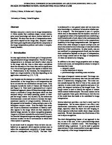
In (17) and (18), two categories of hierarchy are described (see Figure 2): 1. Compositional hierarchy, where lower level properties are constituents of higher level properties. This can be seen to correspond to α-aggregation, the AN D relationship, or part-whole; 2. Specificity or type hierarchy where higher level properties are defined at a lower resolution than lower level properties. This can be seen to correspond to β-aggregation (17, 18), or the OR relationship. We can relate these two categories of hierarchy to the account of micro-macro-property relationships given in (24), which defines a property P1 to be a macro-property of another property P2 if: • P2 has a greater scope than P1 ; • P2 has a lower resolution than P1 ; or • both. The scope of a property is the set of constituents required for the property to exist; for example, the property of being a flock requires a minimum number of birds. On the other hand, the resolution is the set of distinctions that have to be made to distinguish the property; for example, to identify a colour, one needs to be able to distinguish between a ranges of wavelengths. Information-theoretic interpretations of emergence in dynamic systems are based on the idea that often, when we are considering a greater scope, we are willing to accept some loss of accuracy or a lower resolution when predicting future behaviour (see, for example (26) and (4)). Every property in a system or simulation requires a particular scale to be observed; this is also its magnitude defined in terms of that scale. We can recast scale in terms scope and resolution. If we define a scale as a measure of some dimension, the scope is the difference between the maximum and minimum values in that dimension and the resolution is the 4

Figure 2: Two categories of hierarchy. (a) Compositional hierarchy/α-aggregation: P2 , P3 and P4 are constituents of P1 . (b) Type hierarchy/β-aggregation: P6 , P7 and P8 fall in the set defined by P5 .

5

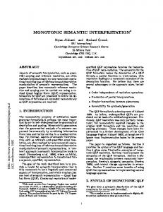
Figure 3: Temporal scale used to observe an agent’s behaviour is recast into scope and resolution. (a) Entity action level resolution but scope is composed of three entity action time steps. (b) Scope is again composed of three entity action time steps but resolution is lower than the entity action level so that the second entity action is not observed. set of distinctions we can make in the dimension. For example, to observe a configuration of entities in area m × n at a given moment of time, we would require a temporal scope of 1 at the time point resolution and a spatial scope of m × n at a resolution at least as fine-grained as the size of the smallest entity. Figure 3 shows how this can be applied to temporally extended behaviours with different temporal scales.

2.4

Multi-level properties

In an agent-based simulation, every computationally distinguishable property consists of one or more (micro-)properties located in an n-dimensional (hyper)space. These can be specified by coordinates e.g. the global coordinate (12, 1, 4, 2) might represent the location 6

of a state transition in the 12th time step (first tuple item holds time), located in coordinate (1, 4) of physical space (second and third tuple items hold space) in component with ID 2 (final tuple item holds component identity). Different coordinate systems can also be used to specify the location of properties with respect to each other e.g. the equivalent coordinate of the above example using a local coordinate system defined with respect to component 2 at time step 11 in the same spatial location would be (1, 0, 0, 0). We can relate this idea to the definitions of levels of abstraction given above: • α-aggregation means that if two macro-properties A and B consist of constituents of the same types and the constituents of the same type have the same organisational relationships with respect to each other, the two properties are of the same type. In terms of location, this means that if the location of one of the constituent properties is taken as the origin of the local cooridnate system and every other constituent is located with respect to it in A, every property in B should have the same coordinates if the corresponding property is taken as the origin. • β-aggregation means that we can describe regions as well as point locations in a system or subsystem space. For example, in a system with only time and identity represented, (before 3, 4) stands for all the states or state transitions that occur in component 4 before time step 3.

3

Multi-level processes as Complex Events

In this section, we introduce our complex event formalism and briefly describe how complex event types can be used to represent multi-level behaviours in agent-based simulations and systems. We then relate compositionality in complex event types to scope, and specificity to resolution. The formalism is also used to express important emergence constructs and definitions more precisely. This allows complex event types to be classified into those that correspond to emergent behaviours and those that do not.

3.1

Events

We define an event as a change in state in an agent-based simulation, where the initial and target states are described at some level of abstraction (see Definition 1). Definition 1 Event. An event is a state transition defined at a particular level of abstraction: e ≡ q1L ⇒ q2L , where • q1L is the initial state described at level L;

7

• q2L is the target state described at level L; and • ⇒ is a state transition function that results from the execution of one or more state transition rules. In many cases, state transition functions can also be decomposed into lower level state transition functions. For example, a state transition function that maps a source subsystem 0 state qSub to another subsystem state qSub (the target state) might be decomposable into a set of lower level subsystem state mappings {(qSub ∗ → qSub ∗0 )}, which can be further 0 )}. If variables are the lowest decomposed into a set of agent state mappings {(qC → qC level of state representation, every state transition function would ultimately be reduced to a set of state transitions mapping a variable value to a new variable value {(var → var0 )}.

3.2

Simple events and complex events

We define a simple event as a state transition that results from the execution of a single state transition rule, and this state transition function can be defined at any level of abstraction. Definition 2 Simple event. A simple event se is a state transition defined at some level of abstraction that results from the execution of a single state transition rule: se ≡ q1L → q2L , where • q1L is the initial state described at level L; • q2L is the target state described at level L; and • → is a state transition function that results from the execution of a single state transition rule. A complex event ce is defined as either a simple event se or two complex events linked by the non-commutative relationship ./ (see Definition 3). Definition 3 Complex event (recursively defined). A complex event is either a simple event se or two complex events ce1 and ce2 satisfying a set of constraints with respect to each other3 : ce :: se | ce1 ./ ce2 3

Constraints can apply to either the events’ source or their state transitions.

8

In a simulation, the relationship ./ might, for example, be a temporal operator ⊗ optionally followed by descriptions of (i) space constraints and (ii) constraints pertaining agent(s)generating the two related complex events. In this example, the syntactic pattern for a complex event relationship ./ would be given by: e1 ./ e2 :: e1 ⊗ [space] [id] e2 where • The temporal constraint ‘⊗’: defines the temporal relationship between e1 and e2 (e.g. e1 must occur after e2); • The spatial constraint ‘space’: defines the space within which e2 should occur relative to e1 (e.g. e1 must occur within distance x of e2) • The agent constraint ‘id’: defines the relationships between agents generating the two events e1 and e2 (e.g. that e1 and e2 must be generated by the same agent).

3.3

Simple and complex event types

We can define a simple event type SET by the two-tuple: SET = (→, Level), where • → is a state transition function that results from the execution of a particular state transition rule; and • Level is the level of abstraction at which the state transition is described. A simple event se has the type SETX iff : • se = q1L → q2L ; • →= A; and • L = B, where SETX = (A, B)

9

→ allows us to distinguish between events resulting from different state transition rules, while Level allows us to distinguish between different levels of observation. A complex event type CET can be defined by the four-tuple: CET = ({SETi }, {CETj }, {./k }, {CETl }), where • {SETi } is a set of simple event types; • {CETj } is a set of complex event types; • {./k } is a set of non-commutative location constraint relationships; and • {CETl } is a set of complex event types. A complex event ce is then said to have the type CETX iff : 1. ce = se and the type of se ∈ A; or 2.

• ce = ce1 ./ ce2 ; • the type of ce1 ∈ B; and • ./∈ C; and • the type of ce2 ∈ D,

where CETX = (A, B, C, D). The type of a complex event is therefore determined both by the types of its constituent events and the relations that hold between them. This definition of a complex event type reflects the hierarchical structure of a complex event since two complex events are only of the same type if they have the same structure4 .

3.4

Hierarchy, Scope and Resolution of complex event types

As described in Section 3.4, two types of macro-micro relationships can be distinguished between properties. The first is the compositional relationship or α-aggregation, where a micro-property is a constituent of a macro-property. The second is the subtype-supertype relationship or β-aggregation, where a micro-property is a subtype of a supertype. In the context of complex event types, we can say that a complex event type CETA is a constituent of a complex event type CETX if: CETX = CETA ./ CETB 4

In practice, it is possible to specify complex event types implicitly via its effects (state transitions).

10

or CETX = CETB ./ CETA . CETX is also said to have a greater scope than CETA . To say that a complex event type CETA is a subtype of a complex event type CETX , the set of events that can be classified as CETA must be a subset of CETX : ECET A ⊆ ECET X . CETX is then said to have a lower resolution than CETA .

3.5

Non-simple complex events as emergent behaviours

In the previous section, we reviewed emergence theories for designed multi-agent systems and distinguished between the designed aspects of the system (LP ART S ) and those aspects of the system that are not designed i.e. can not be generated solely by LP ART S . For behaviours, LP ART S can be seen to correspond to the state transition rules. For a complex event type to represent an emergent behaviour, we therefore require that it contains some constraint that is not included in the state transition rules. This is the case when the complex event type can not be expressed in terms of a single simple event type i.e. it can not be generated from the execution of a single state transition rule.5

3.6

Top-down constraints and emergent ‘laws’

A distinction is often drawn between higher level emergent properties with causal efficacy and those that do not (e.g. (29), (25)). In top-down ‘causation’6 , the presence of a higher level property places constraints on the properties that can be realised at lower levels (e.g. (3)). Since the higher level properties are themselves generated by lower level properties, this can also mean that regularities or ‘laws’ can emerge at higher levels. We formalise these two phenomena in complex event terms: Definition 4 An emergent law exists between two complex event types CETx and CETy when a complex event type CETx exists such that the occurrence of CETx implies the occurrence of some complex event of the type CETy i.e. CETx → CETy , and CETx is not a simple event. 5

An important point to note here is that the distinction between simple and non-simple complex events lies not in the scopes and resolutions of their state transitions, but in their source or origin. Whereas simple events are those that arise from the application of a single state transition rule, the non-simple complex events are those that are either defined at a lower resolution (i.e. include more than one type of simple event) or result from the execution of more than one state transition rule. 6 We prefer to use the term ‘constraint’ rather than ‘causation’ since we make no claims with regard to the ontological or metaphysical status of the epistemologically emergent higher level property or its causal power

11

Definition 5 A top-down constraint effect exists between two complex event types CETM and CETm when an emergent law CETM → CETm holds and CETm is a lower level complex event type with respect to CETM .

3.7

Epistemological equivalence and uniqueness

Two complex events ce1 and ce2 are said to be epistemologically equivalent if for every complex event in ce1, there is a corresponding complex event in ce2 of the same type which satisfies the same constraints on its relations with every other complex event. This is the same as saying they have the same complex event type. Definition 6 Epistemological equivalence of complex events. Two simulations ce1 and ce2 are epistemologically equivalent if (i) they have the same scope and resolution, and (ii) for every complex event cei in ce1 there is exactly one corresponding complex event cej in ce2 of the same type which satisfies the same constraints on its relations with every other complex event in ce2 as cei satisfies with respect to every other complex event in ce1 i.e. ce1 and ce2 have the same complex event type. Definition 7 Epistemological uniqueness. A complex event type CET : CET = ({SETi }, {CETj }, {./k }, {CETl }), is epistemologically unique if any one of the following holds: • {SETi } contains at least one member that is not found in any other complex event type; or • {CETj } contains at least one member that is not found in any other complex event type; or • {./k } contains at least one member that is not found in any other complex event type; or • {CETl } contains at least one member that is not found in any other complex event type.

4

Formulating and computationally testing multi-level hypotheses

In practice, agent-based simulations tend to be used to validate hypotheses about the behaviour of the system as a whole (the collective behaviour of the agents), given the set of rules of the ABM. Because the collective behaviour is often not analytically derivable from the agent rules and arises only when agents interact dynamically in a common environment, 12

simulations have been called ‘opaque thought experiments’ (20), (2). In such studies, the behaviour of the whole system is typically represented by a macro-state variable that aggregates the states of all the agents in some way; this macro-state variable is then tracked through time. A major problem with this approach is the loss of structure when states are aggregated e.g. no information about spatial locality is retained. This means that we are unable to identify the mechanisms (the actual interactive patterns between agents) that give rise to a particular global behaviour. For this reason, simulations are usually visualised, allowing the human experimenter to observe visually the interactions taking place through time. Hypotheses about such interactions are then formulated in natural language and hence vague e.g. ‘the cells cooperate to survive’. The complex event formalism gives us a means to formally express such hypotheses in terms of the agent-based model. Once expressed formally, we can then identify the particular interactive mechanisms or classes of mechanisms in simulation, giving us a computational method for testing such hypotheses. A simple illustration of this is given below for a set of Game of Life simulations. Our study is simple, but it demonstrates how multi-level hypotheses about the model can be formulated and tested empirically with simulation using our formalism. We also study the relationship between initial condition differences and higher level behaviours. We give the rules for the game of life in ABM terms, where each element is an agent of the same type in one of two states, dead (D) or alive (A). The rules are as follows: 1. Death by loneliness: If A ∧ (n ≤ 1), A → D; 2. Death by overcrowding: If A ∧ (n > 4), A → D; 3. Stay alive: If A ∧ (n == 2 ∨ n == 3), A → A; 4. Resuscitate: If D ∧ (n == 3), D → A 5. Stay dead: If D ∧ (n! = 3), D → D, where n is the number of neighbours in state A.

4.1

Specifying complex event types

In our study, we wish to answer the following questions: 1. Which of two oscillitary mechanisms is more dominant in keeping the system ‘alive’ (see below for definition)? 2. What effect does the initial number of live cells have on the ability of the system to stay ‘alive’ ? 3. Is there a relationship between the initial number of live agents and the degree to which an oscillator is observed?

13

We consider the system to be alive so long as at least one of its cells is evolving (undergoing a state transition); once this is no longer the case, the system is considered dead since it can no longer evolve. The extent to which a system stays alive during the course of the simulation is therefore measured by the length of time for which this is true. We can specify the complex event type for staying alive SA as: SA = (∅, A, {; , [a 6= b]}, B), a ∈ A, b ∈ B where A and B are sets containing every complex event type that can be generated by the model, ; is the temporal operator indicating that an event of type A must immediately follow one of type B, and the constraint A 6= B stipulates that A and B must be different types. In this study, we try to determine which of two oscillators are dominant in keeping systems alive by specifying them as complex event types and then measuring their occurrence throughout the system’s lifetime7 Figure 4 shows the two types of 2-period oscillators and their complex event types. Due to space limitations, we are unable to give the full specifications for the complex event types HV , V H, C or E, but Figure 4 gives a diagrmmatic representation of them. The complex event types representing the two oscillators respectively are therefore: O1 = (∅, X, {; , [x 6= y]}, Y ), x ∈ X, y ∈ Y, where X, Y = {V H, HV } and O2 = (∅, P, {; , [p 6= q]}, Q), p ∈ P, q ∈ Q, where P, Q = {E, C}.

4.2

Results and interpretation

In the simulation study, we investigate the effects of changing the initial number of live agents n. First, we try to establish whether n makes a difference to the system’s lifetime SA by comparing the mean simulation time for each of the n values (again, the maximum value for SA is 100). Table 1 summarises the results for the different n value simulation groups. An analysis of variance (ANOVA) for t between the three groups gave an F value of 0.737 with p = 0.480, indicating that there is no significant difference between the three groups in system lifetime. We then try to establish whether n affects the extent to which oscillator 1 is exhibited8 . An ANOVA indicated no significant difference (F = 1.026, p = 0.361) between groups, from 7

In a more extensive study, a greater number of oscillators, gliders etc. would need to be specified. We ignore oscillator 2 in this analysis, since its occurrence was so infrequent (only once during all 150 simulations). 8

14

Table 1: Summary statistics for simulations with different n values (initial number of live agents). rSA−O1 = correlation between SA and O1; rSA−O2 = correlation between SA and O2; p = probability of the r value occurring by chance (0.05 significance). All values given to 3 decimal places.

mean SA sd SA mean O1 sd O1 mean O2 sd O2 rO1−SA pO1−SA rO2−SA pO2−SA

n = 25 55.900 36.538 30.240 85.110 0.000 0.000 0.416 0.003 (sig.) n/a n/a

n = 50 64.020 34.893 13.160 25.560 0.020 0.141 0.477 0.000 (sig.) 0.145 0.316 (not sig.)

n = 75 62.480 35.094 24.720 56.707 0.000 0.000 0.381 0.006 (sig.) n/a n/a

which we can conclude that the number of live agents at the beginning the simulation does not in itself determine the extent to which the oscillator is exhibited. Across all groups, there was a significant positive correlation between the degree to which O1 occurred and SA but not between the degree to which O2 occurred and SA (since O2 was exhibited so infrequently). Returning to our original questions, we can summarise our findings as follows: 1. Overall, Oscillator 1 is more dominant in keeping the system. 2. For the different values of n we used, the initial number of live cells has no effect on the ability of the system to stay alive. 3. For the different values of n we used, there is no relationship between the number of live agents and the degree to which an oscillator is observed. But what does it mean to say there is no significant difference between groups defined by different n values? Each unique simulation for a given value of n is a member of the population of all possible simulations that can be generated by the model given the value of n. Effectively, the parameter n determines the probability of certain configurations being realised and it is these initial configurations that determine whether or not certain oscillatory behaviours will occur. When we say that there is no difference between groups with different n values with respect to a particular behaviour, we mean that differences in initial configuration are not important in determining whether the behaviour occurs. 9 9

It is likely that if a greater range of n values were investigated, there would come a point where the

15

5

Agent-based models as functions that generate complex event types

An agent-based model (ABM) is both a generator and a classifier of simulations. All the simulations that can be generated by the same ABM lie within a common set. More formally, we can define an ABM as a function which takes the arguments: Agents, a set of agents a0 , ..., an , and Conf ig, a configuration defining the initial conditions (e.g. where each agent is situated, global and local variable values, random seed values, simulation time etc.), and returns the simulation: ABM (Agents, Conf ig) = SimABM ,

(1)

where M ember(SimABM , ABM ) = true. i.e. SimABM belongs to the set of simulations that can be generated by the model ABM . (Environmental objects, shared data spaces, global and local variables etc. are all members of Agents in this definition.) In complexity science, ABMs are usually parametised; these parametised versions of the ABM can be treated as sub-types of the ABM, since they represent more specific models, which again define a set of simulations (see Figure5). So we can define a parametised ABM as a model that given the ABM and a particular set of parameters P , returns a simulation: P aramABM (ABM, P ) = SimP aramABM , where M ember(SimP aramABM , P aramABM ) = true. Similarly, each agent type Ai is a generator and classifier of agents (instances of a type): A(c) = a, where a is an agent instance of the type A, c is the initial state of the agent, and M ember(a, A) = true Agents and simulations are both complex events (see Figure 6). An agent in simulation is a series of simple events (with the constraint that they take place in the same agent) while a simulation is simply a network of simple events where each simple event satisfies a set of constraints relative to every other simple event. n value would begin to result in significantly different systems with respect to the oscillatory behaviours considered.

16

6

Defining the epistemological limits of an agent-based model

The epistemological limits of an agent-based model is the knowledge that we can theoretically gain from the model’s simulations10 . This is defined both by the set of epistemologically unique simulations that can be generated by the model and the set of unique hypotheses that can be computationally tested.

6.1

Assumptions about the limitations of computation

There are two key limitations of computational representation that have important consequences for the epistemological limits of simulations. 1. Simulations can not be infinite since computational power is finite; 2. True randomness can not be represented. Random behaviour can only be simulated by a pseudo-random generator with a given seed. The epistemological consequences of these two limitations when considered in the context of our theory of agent-based simulation are described below.

6.2

The set of epistemologically unique simulations that can be generated

Since a simulation is a complex event, at a particular level of abstraction two simulations sim1 and sim2 are epistemologically equivalent if for every complex event in sim1, there is a corresponding complex event in sim2 of the same type which satisfies the same constraints on its relations with every other complex event i.e. they have the same complex event type. From Definition 6, it is also clear that epistemological equivalence is dependent on the resolution at which complex events are observed or described (the resolution of the complex event type). Two simulations (or complex event types) may have epistemological equivalence at one resolution but not at a higher resolution. However, each ABM itself defines a maximum resolution for its simulations. Agent rules define the maximum resolution for an event source while the highest resolution for state transitions is determined by the state variables used. This is the maximum resolution at which epistemologically unique complex event types can be specified. Because neither infinity nor randomness can truly be represented computationally, the set of possible initial condition configurations Conf ig (see Equation 1) is finite, and each configuration generates a simulation that has an epistemologically unique complex event type. Since the set of possible initial condition configurations {Conf ig} is finite and the only simulations that can be generated by the ABM are those from {Conf ig}, the set of epistemologically unique complex event types that ABM can generate is finite. 10

NB. This is not the same as the knowledge we can gain about the system being modelled using the ABM and its simulations.

17

6.3

The set of hypotheses that can be computationally validated

A hypothesis can be computationally validated by simulation if, by executing any subset of the ABM’s epistemologically unique simulations, it is possible to determine whether or not the hypothesis is true. A hypothesis can be formulated at any level of abstraction (within the limits defined by the ABM, see above) using a first order predicate formula with complex event type variable(s) and predicates relating complex event types (e.g. CET1 [occurs more frequently than] CET2 , CET1 [always occurs at the same time as] CET2 ...). Since both the set of predicates and the set of epistemologically unique complex event types is finite, the set of hypotheses that can be computationally validated is finite.

7

Summary and Conclusions

In this presentation, a formalism has been proposed that is able to describe any computationally distinguishable property in an agent-based simulation. The complex event formalism is based on the Process Philosophy of Whitehead (35) but is formulated in terms of multi-level agent-generated events in simulations. As a contribution to the practice of agent-based modelling and simulation, specification of complex event types provides us with a novel computational method for validating multi-level hypotheses (Section 4). More important theoretically however, the formalism has given us the means to precisely define a theory of agent-based simulation, and establish the epistemic limits of any given agent-based model. This can be summarised as follows: 1. An ABM is an implicit specification for a complex event type CETABM . 2. Each parametised ABM is a subtype of CETABM . 3. Every epistemologically unique simulation is an epistemologically unique complex event type that is a subtype of CETABM . 4. A hypothesis that can be computationally tested is one that can be expressed in terms of a first order predicate formula with at least one epistemologically unique complex event type variable. 5. Because computational representation is finite, both the set of epistemologically unique simulations and the set of hypotheses that can be computationally tested for an ABM are finite, establishing the epistemological limits of the ABM. Formalisation of computational practices in this way brings clarity to the philosophical debates surrounding them. In the current discussion, we have established that the finite nature of ABMs’ epistemic limits derive from the inability of computers to represent infinity and/or true randomness. A serious dialogue between Philosophy and Computer Science is required to establish what implications this has for the methodological, epistemological, 18

and perhaps even metaphysical status of agent-based simulations. Yet it is only through the explicit and precise formulation of a theory for agent-based simulation that we have been able to pinpoint where the key issues lie.

Acknowledgements I am supervised by Christopher D. Clack, Department of Computer Science, University College London and Sylvia B. Nagl, Department of Oncology, UCL Cancer Institute and UCL Research Department of Structural and Molecular Biology. I would also like to thank Richard Hawkins and James Driscoll, Department of Philosophy, University of Oxford, who taught me Philosophy of Science, Philosophy of Psychology and Philosophy of Mind during my undergraduate degree.

References [1] R. Axelrod. The Complexity of Cooperation: Agent-based models of Competition and Collaboration. Princeton University Press, 1997. [2] M. A. Bedau. Downward causation and the autonomy of weak emergence. Principia, 3:5–50, 2003. [3] R. D. Beer. Autopoiesis and cognition in the game of life. Artificial Life, 10:309–326, 2004. [4] E. Bonabeau and J. L. Dessalles. Detection and emergence. Intellectica, 2(25):85–94, 1997. [5] F. Boschetti, M. Prokopenko, M. Macraedie, and A. Grisogono. Defining and detecting emergence in complex networks. In R. Khosla, R. J. Howlett, and L. C. Jain, editors, Knowledge-based intelligent information and engineering systems, 9th International Conference, KES, volume 3684 of LNCS, pages 573–580. Springer, September 2005. [6] C-C. Chen, S. B. Nagl, and C. D. Clack. A calculus for multi-level emergent behaviours in component-based systems and simulations. In M. A. Aziz-Alaoui, C. Bertelle, M. Cosaftis, and G. H. Duchamp, editors, Proceedings of the satellite conference on Emergent Properties in Artificial and Natural Systems (EPNACS), October 2007. [7] C-C. Chen, S. B. Nagl, and C. D. Clack. Specifying, detecting and analysing emergent behaviours in multi-level agent-based simulations. In Proceedings of the Summer Simulation Conference, Agent-directed simulation. SCS, 2007. [8] C-C. Chen, S. B. Nagl, and C. D. Clack. A method for validating and discovering associations between multi-level emergent behaviours in agent-based simulations. In 19

Proceedings of the second international symposium on agent and multi-agent systems: technologies and applications, LNAI 4953. Springer, March 2008. [9] V. Darley. Emergent phenomena and complexity. Arificial Life, 4:411–416, 1994. [10] R. Frigg and J. Reiss. The philosophy of simulation: Hot new issues or same old stew? Synthese, 2008. [11] P. Grassberger. Toward a quantitative theory of self-generated complexity. International Journal of Theoretical Physics, 25:907–938, 1986. [12] V. Grimm, E. Revilla, U. Berger, F. Jeltsch, W. M. Mooij, S. F. Railsback, H-H. Thulke, J. Weiner, T. Wiegand, and D. L. DeAngelis. Pattern-oriented modelling of agent-based complex systems: Lessons from ecology. Science, 310:987–991, November 2005. [13] S. Hartmann. The world as a process: Simulation in the Natural and Social Sciences, pages 77–100. 1996. [14] S. Hokky and Y. Surya. Agent-based model construction in a financial economic system. In Proceedings of the Conference of New Economics Window, 2004. [15] P. Humphreys. Computational science and scientific method. Mind and Machines, 5:499–512, 1995. [16] K. Izumi and K. Ueda. Emergent phenomena in a foreign exchange market: Analysis based on an artificial market approach. In C. Adami, R. K. Below, H. Kitano, and C. E. Taylor, editors, Artificial Life VI, pages 398–402. MIT Press, 1998. [17] J. Johnson. Hypernetworks for reconstructing the dynamics of multilevel systems. In Proceedings of European Conference on Complex Systems, November 2006. [18] J. Johnson. Multidimensional Events in Multilevel Systems, pages 311–334. PhysicaVerlag HD, 2007. [19] A. Kubik. Toward a formalization of emergence. Artificial Life, 9:41–66, 2003. [20] E. A. Di Paolo, J. Noble, and S. Bullock. Simulation models as opaque thought experiments. In Artificial Life VII: The Seventh International Conference on the Simulation and Synthesis of Living Systems, Reed College, Portland, Oregon, USA, August 2000. [21] D. Polani. Emergence, intrinsic structure of informatio, and agenthood. In International Conference on Complex Systems (ICCS), 2006.

20

[22] F. Rohrlich. Computer simulation in the physical sciences. PSA 1990 II, pages 507– 518, 1991. [23] E. Ronald and M. Sipper. Design, observation, surprise! a test of emergence. Artifcial Life, 5:225–239, 1999. [24] A. Ryan. Emergence is coupled to scope, not level. Nonlinear Sciences, 2007. [25] R. K. Sawyer. Simulating emergence and downward causation in small groups. In Proceedings of the Second International Workshop on Multi-Agent Based Simulation, pages 49–67, Berlin, 2001. Springer-Verlag. [26] C. Shalizi. Causal Architecture, Complexity and Self-Organization in Time Series and Cellular Automata. PhD thesis, University of Michigan, 2001. [27] C. R. Shalizi. Methods and Techniques of Complex Systems Science: An Overview, chapter Methods and Techniques of Complex Systems Science: An Overview, pages 33–114. Springer, New York, 2006. [28] C. R. Shalizi, K. L. Shalizi, and R. Haslinger. Quantifying self-organisation with optimal predictors. Physical Review Letters, 93(118701), 2004. [29] M. Silberstein and J. McGeever. The search for ontological emergence. The Philosophical Quarterly, 49(195):201–214, 1999. [30] S. Sismondo. Science in Context, 12:247–260, 1999. [31] M. Stockler. On Modelling and Simulations as instruments for the study of Complex Systems. University of Pittsburgh Press, 2000. [32] J. C. Tay and A. Jhavar. A complex adaptive framework for immune system simulation. ACM Symposium of Applied Computing, pages 158–164, 2005. [33] L. Tesfatsion and K. Judd. Handbook of Computational Economics 2: Agent-based Computational Economics. Elsevier, 2007. [34] D. C. Walker, J. Southgate, G. Hill, M. Halcombe, D. R. Hose, S. M. Wood, Mac Neil, and R. H. Smallwood. The epitheliome - agent-based modelling of the social behaviour of cells. BioSystems, 76:89–100, 2004. [35] A. N. Whitehead. Process and Reality. Free Press, 1978.

21

Figure 4: Two 2-period oscillators and their complex event types (see text for the state transition rules associated with the indices). A = black, D = white. For the complex event types, the grid represents the spatial relations that these events must have with each other at a single time point. (a) oscillator 1 O1 can be either the complex event type V H (vertical to horizontal) or the complex event type HV (horizontal to vertical); (b) oscillator 2 O2 can be either the complex event type E (expand) or C (contract).

22

Figure 5: An agent-based model (ABM) generates a population of simulations, SimT otal . Different parametisations/initial conditions etc. of the ABM can be regarded as different models X, Y..., each of which generate a population of simulations SimX , SimY ... ∈ SimT otal . These are subsets of the population of simulations generated by the ABM.

23

Figure 6: A simulation is a complex event which can be decomposed in different ways. These different decompositions can be expressed in terms of complex event types.

24