The dynamics of flame spread on these objects is made considerably more complex by the fact that these materials melt and flow at elevated temperatures. The.
A PROGRESS REPORT ON NUMERICAL MODELING OF EXPERIMENTAL POLYMER MELT FLOW BEHAVIOR Kathryn M. Butler, Thomas J. Ohlemiller, & Gregory T. Linteris National Institute of Standards and Technology, USA
ABSTRACT A combination of experiment and modeling is being used to investigate the effects of material properties on the melt flow behavior of thermoplastics. The dripping behavior of several types of polypropylene has been studied, including measurements of mass loss from the sample and mass collection in the catchpan, surface temperature, and surface velocities. An experimental method was developed for extrapolating viscosity data to high temperatures where bubbles in the polymer make standard rheometry impossible. A finite volume model that uses the volume of fluid method to track the highly distorted interface for a melting and dripping polymer is described. The model includes heat flux to the distorted interface, empirical viscosity as a function of temperature, flow due to gravity, and gasification. INTRODUCTION Many objects contained in buildings, including mattresses, electronic housings, some furniture, and fabrics, behave as thermoplastics in fire. The dynamics of flame spread on these objects is made considerably more complex by the fact that these materials melt and flow at elevated temperatures. The flow greatly affects heat and mass transport and the shape of the fuel changes during the course of the fire. Widely divergent effects may follow. If the melted polymer pool does not sustain ignition, the flow will transport flammable material away from the fire and reduce the fuel load. If the melt pool does ignite, the flow provides a significant mechanism for fire spread. Fire experiments on vertically oriented thermoplastic samples by Zhang et al.1 demonstrated that the flame spread was eventually dominated by the pool fire that formed at the base. Sherratt and Drysdale2 confirmed this result and also showed that the type of flooring material is an important variable in pool fire development. In a study (to be published) of fire spread on thermoplastic computer monitor enclosures, Bundy and Ohlemiller found that, with a variety of polymer resins, interaction between the melt fire on the catch surface and the fire on the monitor sides greatly influences the dynamics of the spread.3 In previous work4,5, a model for polymer melting was compared to experimental results for non-gasifying polymer flow. The experiments tested low molecular weight (MW) atactic polypropylene (PP) samples at a range of incident radiant heat fluxes. The low viscosity of the atactic PP caused flow of the material at sufficiently low temperatures that the polymer did not degrade; 100 % of the original mass was recovered in the catch pan. The mass loss rate predicted by the model agreed to within 20 % for this material. This paper reports the work done to date on an extension of the comparison of model and experimental results to thermoplastics that undergo degradation at high temperatures. METHOD A combined experimental and modeling effort is underway to clarify the role of the properties of thermoplastics in their burning behavior, including the effects of flow. While most full density thermoplastics in consumer products are in the form of thin-walled, mold-shaped objects, this study has focused first on simple planar, thermally thick vertical slabs heated radiatively on one face only. This simplification precludes bulk collapse of the sample and places the emphasis on the melt flow process
from the heated face and its competition with gasification. In addition, the problem addressed at this stage excludes burning, though not gasification; flames will be added at the next stage of study. Experimental A schematic of the apparatus used in this set of experiments is given in Figure 1. A polymeric sample is mounted vertically and exposed to uniform radiant heating on one face from a Cone heater placed on its side. The sample measures 2.5 cm thick by 5 cm wide by 10 cm tall and is insulated on its lateral edges and back surface. The NIST calorimeter,6 slightly modified, was used for the tests. In addition to the sample load cell typically used, a laboratory balance (Mettler PE3607) was added below the sample to weigh the mass of dripping polymer as a function of time. The cone test area was enclosed in an approximately air-tight aluminum shroud (with a viewing window), and dilution nitrogen at laboratory temperature was added around the catch pan and directed upward to eliminate the possibility of ignition of the polymer decomposition gases from the surface of the hot cone radiant heater. A cylindrical aluminum foil tube (2.5 cm diameter, 15 cm tall) caught the dripping polymer so that the time sequence of the melt could be approximately preserved. Additional discrete grab-samples (typically two or three) were obtained with 2.5 cm diameter, 6 mm tall foil pans inserted into the dripping stream. A fine-wire thermocouple (Omega type K, 0.13 mm diameter) was traversed through the melt layer, and the maximum indicated temperature was taken as the surface temperature. Kapton7 film particles (1 mm square) were injected onto the melt surface with a small flow of air carrier gas, and their motion was tracked via video images of the melt process (30 Hz framing rate). This provided estimates of the melt surface velocity as a function of time during the test and position on the sample. Figure 1.
Gas Fired Radiant Panel
Polymer Melt Apparatus 2.5 cm Thick Polymer Sample in Frame (Edges and Rear Face Insulated)
SCALE
Polymer Melt Forming Pool
SCALE
Several formulations of polypropylene have been studied using this type of apparatus. PP23K is a waxlike formulation that flows off the sample surface at such a low temperature that it can be modeled without the complication of gasification chemistry. Polypropylene type PP6523 is a high viscosity commercial injection molding resin formulation. Polypropylene type PP702N is a low viscosity commercial injection molding resin formulation. At normal processing temperature (ca. 230 °C) these latter two resins differ in melt viscosity by about a factor of nine. The viscosity of the PP23K is an order of magnitude greater than that of PP6523.
Viscosity is a key determinant of the melting behavior of thermoplastic materials. The characterization of viscosity as a function of experimental parameters under these test conditions is a difficult challenge. Viscosity is a function of molecular weight as well as temperature. As a polymer is heated well above normal processing temperatures, chemical bonds are broken, resulting in shorter polymer chains and a widening of the molecular weight distribution. Sufficiently small polymer fragments can nucleate and gasify. At the temperatures reached in a fire, thermal degradation of polypropylene and many other polymers generates bubbles within the melt that confound standard polymer melt viscosity measurement techniques. To address this problem and to provide a simple viscosity-temperature relationship for modeling purposes, a unique experimental method is used. Samples of the melt generated at measured temperatures during the dripping experiment of Figure 1 are collected. The molecular weight distribution of these samples is presumably fixed upon cooling. A Paar Physica rheometer is used to measure the viscosity of each sample with temperature up to the point at which bubbling begins. The sample is bathed in nitrogen during the measurement, which is performed at a heating rate of approximately 1 °C/min and shear rate of 1 s-1. Rheometry is also used to characterize the temperature-dependent viscosity of the original resin well upward in temperature to the point where bubbling begins. It is this curve that requires extrapolation to the surface temperatures seen in the melt experiments. Viscosity measurements on the collected melt samples provide points on the extrapolated curve (a single viscosity value at each measured surface temperature). The net result is an empirical viscosity-temperature curve that covers the full temperature range of interest and implicitly incorporates molecular weight changes. This technique is approximate in that it ignores residence time issues at any given temperature, which could, in principle, affect the extent of degradation. The chemical kinetics used to model gasification are determined through experiment. The weight loss kinetics are obtained from thermogravimetric measurements consisting of triplicate TGA runs at heating rates of 0.5, 2, and 5 °C/min. The Kissinger method is applied, using the assumption of the first order weight loss rate law d/dt(w/w0) = A (w/w0) exp (-E/RT)
,
[1]
where w0 is initial weight, A is the pre-exponential factor, E is the activation energy, R is the universal gas constant, and T is temperature in kelvins. The Kissinger method utilizes the shift in fractional weight loss with heating rate to infer the effective activation energy of the overall weight loss process and the pre-exponential factor. Thermal conductivity of the polymers under investigation was measured using a commercially-available apparatus based on transient heating for temperatures from 40 °C through 265 °C. Modeling The melt flow behavior of thermoplastics involves large changes in geometry over time. This suggests a finite element or finite volume approach, in which the domain is divided into discrete cells for calculation of variable values at cell nodes or centers. These approaches are designed to handle complex geometries and incorporate techniques to track the motion of free surfaces. Commercial software packages add modeling flexibility through user subroutines, which provide access to solution variables and allow the user to modify the software for a specific application. Although the necessary computational tools for this problem are ostensibly available in current commercial software, the difficulties encountered during the use of two commercial codes indicate that this application pushes the state-of-the-art. In this paper, development of a model of melt flow behavior using the commercial finite volume software CFD-ACE+7 is described. The numerical model geometry is shown in Figure 2. The problem is 2-D, with the initial sample filling a rectangle 10 cm high by 2.5 cm thick (the purple region). The problem space is 10.3 cm by 3.5 cm to allow the melting sample to overflow the rectangular area as it flows down over the bottom lip. The number of cells in the horizontal or x direction is nominally 40 through the polymeric sample and 16
through the gas region. The number in the vertical or y direction is 50 through the sample, with variable cell heights to make cells nearly square in the region where polymer will flow over the lip and taller at the top of the model where motions are expected to be primarily downward. The boundaries above, to the right, and below the initial sample are fixed walls, with velocities set to zero and adiabatic heat flux conditions. The upper boundary adjacent to the initial sample is an inlet and the lower boundary below the bottom lip is an outlet, with pressure for both fixed at standard ambient conditions. A heat flux is applied directly to the vertical surface of the sample. The left boundary of the problem is assigned symmetry conditions, so that velocity and temperature gradients are zero. Figure 2. Model geometry showing fill variable. The full geometry is shown on the left, and a closeup of the bottom lip region is shown on the right.
Because of the large changes in shape of the thermoplastic sample during the melting and dripping process, the model uses a volume-of-fluid (VOF) method. This method uses a marker concentration field variable, referred to as the volume fraction or fill variable and denoted by F, to delineate the free surface. The variable F is set to unity within the polymer and to zero outside, with the free surface located by steep gradients in this variable, as shown on the right in Figure 2. The problem is embedded in a fixed finite element grid, in which F evolves according to a passive transport equation. As implemented by CFDACE+, two sets of material properties are provided: gas properties for Fluid 1 with F=0, and polymer properties for Fluid 2 with F=1. For cells with intermediate values of F between 0 and 1, contributions from the two fluids are linearly proportional. The solution procedure in CFD-ACE+ solves the volume fraction equation along with equations of mass, momentum, and energy to determine the new locations of free surfaces. The method requires the free surface to cover less than a cell width in a single timestep, which is normally taken care of through the selection of an automatic timestep option. The VOF procedure is capable of tracking a fluid through gross distortions of shape, including breakup and coalescence. This problem requires application of a heat flux to the changing surface of the polymer. The approach taken by the finite element package FIDAP7,8 to model heat or mass transfer at the volume fraction interface is used. In this approach, the heat flux is treated as an equivalent volume source Su added to the energy equation for a cell i, Su = 2 q |∇Fi| Vi ,
[2]
where q is the heat flux, which may include radiative and convective heat loss terms, and Vi is the volume of the cell. CFD-ACE+ provides a user subroutine usource that enables the addition of a source term for any equation at any computational cell. The cell temperature, temperature gradient, and the volume
fraction value and its gradient are accessible to the subroutine. Since the gradient of F is nonzero only in the cells adjacent to the free surface, the source is applied only to the interface. Unphysical heating of the gas next to the polymeric interface is prevented by limiting the volume source to cells in which F is greater than 0.5; the factor 2 in source Su maintains the correct total heat flux. The viscosity of the material depends on temperature and molecular weight. Since molecular weight is not a variable of the model, the experimentally-determined relationship between viscosity and temperature described in the previous section is applied. At low temperatures, the viscosity is set sufficiently high that no appreciable flow occurs. As the heat flux raises the temperature within the sample, its viscosity decreases, and a gravity force applied to the model causes the heated material to flow. The empirical relationship of melt viscosity with temperature is entered into the model through a user subroutine. The transport of heat through the material by conduction results in a large gradient of temperature near the polymer-gas interface. Since polymer viscosity is a strong function of temperature, at any given time only a thin layer of material may actually be flowing. Resolution of this flow layer places an upper limit on the spatial step size. In addition to the flow of material out through the bottom of the computational volume, the polymer also loses mass due to gasification. The chemistry of gasification is described as an Arrhenius function of temperature with kinetic parameters obtained from experiment and occurs in-depth, not just at the surface. The gases are assumed to leave the polymer instantaneously as soon as they are generated, neglecting the messy behavior that arises when bubbles are generated. (Experimentally, few bubbles are seen with the polypropylene resins studied.) Within the CFD-ACE+ model, gasification is represented by the removal of Fluid 2, the polymer, using the user subroutine usource to add sink terms both to Fluid 2 mass and to energy equations for cell i: Fluid 2
Su = - ρA exp (-E/RTi) Vi
Energy
Su = - HvρA exp (-E/RTi) Vi
[3]
,
,
[4]
where ρ is polymer density and Hv is heat of vaporization. The sink terms are added to every cell in the polymer, for which F > 0.5. For the current melt flow problem gas generation is not necessary, but it can be included in this model through a source term for the Fluid 1 (gas) mass equation. The total quantity of gas generated in a time step is equal to the total amount of polymer gasified. The first step in adding gas to the problem is therefore to sum the sink terms for every Fluid 2 cell as given in equation (3). The gas should be added to the problem only at the polymer-gas interface. The cells that will receive a Fluid 1 source term are therefore gas cells, with F < 0.5, adjacent to the interface, having a nonzero gradient of F. Counting these cells and dividing the total quantity of gas by the number of cells, finally, gives the amount of gas to be added to each of these cells. Although a user subroutine can be used to customize any material property, all properties other than viscosity have thus far been kept constant. RESULTS Experimental Figure 3 illustrates the mass lost from the sample and mass collecting in the catch pan for PP702N polypropylene at two heat flux levels. These heat flux values are of the level expected from flame feedback in a vertical wall burning process.9 The difference between the two measures of mass represents the mass loss due to gasification, with a caveat. The plateaus in the drip mass represent melt samples that were removed for viscosity measurements, so a correction needs to be made for the mass of these samples.
Figure 4 shows the velocities experienced by the Kapton particles as they flow with the melt. Each line represents a single particle (two particle trajectories for the upper figure, three for the lower; the darker symbols denote later times in the experiment). The surface temperatures are about 370 °C for 30 kW/m2 and 415 °C for 40 kW/m2. Similar data were collected for PP6523. Figure 3. Mass lost from sample (blue) and mass gained by catch pan (green) for PP702N polypropylene exposed to heat fluxes of 30 and 40 kW/m2.
Figure 4. Velocities measured for Kapton particles on surface of PP702N melt. The top plot is for 30 kW/m2 and the bottom plot is for 40 kW/m2.
Figure 5 shows the viscosity measurements made on the PP702N formulation of polypropylene. Note that the vertical axis encompasses six orders of magnitude. This figure illustrates the interpolation/extrapolation of the viscosity measurements to estimate the melt viscosity from low temperatures up to the surface temperatures measured during the melt flow experiments of Figure 1. The highest curve on the plot is viscosity vs. temperature for the initially undegraded polymer; its downward bend at about 300 °C is due to the onset of degradation. At around 360 °C the polymer begins to gasify, and the rheometer is unable to measure viscosities at higher temperatures. Curves are also shown for two samples of polymer melt collected from the experiments of Figure 1. These also can only be measured up to the point where bubbling begins. The viscosity curve for each sample from one of the two heat flux levels is then extrapolated linearly to the surface temperature at which the sample was formed. The extrapolated points, labeled A for the sample exposed to 30 kW/m2 and B for the 40 kW/m2 sample, are thus used to extend the viscosity-temperature relationship for the polymer to the higher temperatures it encounters when it sees flame level heat fluxes. A similar analysis performed on the PP6523 polypropylene extends the viscosity curve for this polymer to 425 °C. It was found experimentally that this latter polymer, which has a higher initial viscosity, yields a lower viscosity melt at these elevated temperatures. Figure 5. Viscosity vs. temperature for initially undegraded PP702N polypropylene and for melt samples collected from 30 kW/m2 and 40 kW/m2 heat flux exposures. Extrapolation of viscosity to high temperatures is indicated by the black line.
Kinetic parameters for weight loss rate of the polypropylene samples investigated in this study are given in Table 1. The values for types PP702N and PP6523 are obtained from TGA measurements using the Kissinger method. The values used for the low molecular weight PP23K sample are from a molecular dynamics simulation.10 Table 1. Polymer Type PP702N PP6523 PP23K
Activation Temperature E/R (K) 24400 26000 26200
Pre-exponential Factor A (s-1) 2.18 x 10¹² 2.23 x 10¹³ 2.4 x 10¹⁴
Thermal conductivities for the two polymer types were measured for temperatures ranging from 40 °C through 265 °C. Values for type PP702N ranged from 0.24 to 0.28 W/m-K below 150 °C then dropped to 0.22 to 0.24 W/m-K at higher temperatures as the crystalline portion of the polymer melted. Thermal
conductivity for type PP6523 increases slowly with temperature from 0.19 W/m-K to 0.22 W/m-K. As an aside, tests of thin sheets (0.32 cm, 1/8 inch thick) of PP and other commercial thermoplastic resins in a similar apparatus, but with burning, demonstrate the complexity of physical behavior of thin samples in a fire. Samples of ABS, polycarbonate, and polystyrene (HIPS) were observed to bubble and fall from the holder in irregular globs after complex slumping processes, which had a major effect on the rate of heat release. Modeling To demonstrate the capabilities of the VOF approach and the drastic changes in the shape of the sample, previous results4, 5 for flow without gasification using the FIDAP finite element code are reproduced here. A sequence of images showing the time evolution of the free surface of the dripping sample is shown in Figure 6, with the corresponding loss of mass with time in Figure 7. The mass loss rate predicted by the model agreed to within 20 % for this material (PP23K) at three values of heat flux. Figure 6. Time sequence of free surface location for low MW PP23K exposed to 25 kW/m2 heat flux. Sequence shows 100 s intervals from 0 to 700 s.
Figure 7. Fraction of initial mass remaining in sample vs. time for PP23K exposed to 25 kW/m2 heat flux.
The requirement that the volume fraction interface never move more than a single element in one timestep caused the automatic time-stepping mechanism to set the timestep on the order of a few milliseconds once flow started. This caused this job to take a few days to run. Attempts to add gasification to this problem ran into difficulties with spurious high velocities and instabilities in the volume fraction interface. At this point a move was made to CFD-ACE+ software. A sequence of problems was solved in order to determine the best solution parameters, try different boundary conditions, and test the behavior of the model. The first test problem considers a steady state flow with constant viscosity in the presence of gravity. The computational space is the polymeric sample only, with a fixed wall on the right, symmetric boundary conditions on the left, and fixed (and equal) pressure inlet and outlet conditions on the top and bottom respectively. The resulting parabolic velocity profile is shown in Figure 8. Figure 8. Gravity-driven flow with constant viscosity.
The second set of problems looks at the application of a heat flux to the volume fraction interface. To speed up the investigation of basic capabilities of the CFD-ACE+ software, a smaller test problem was set up with 40 cells in the polymer and 8 cells in the gas in the x direction and 10 cells in the y direction. The grid is displayed in Figure 9 along with temperature shading for a fixed wall with adiabatic boundary conditions on the left face. The right face is a fixed wall and upper and lower boundaries are adiabatic so that the problem is one-dimensional. No flow is allowed. The heat flux applied to the volume fraction interface includes radiative and convective losses, q = αq0 – εσ(T4-T04) – hc(T-T0), where α is absorptivity, ε is emissivity, σ is the Boltzmann constant, and hc is the convective coefficient. For calculation purposes, the temperature T accessed by the user subroutine is the value for the cell center adjacent to the interface.
Figure 9. Temperature shading at t=100 s for fixed wall boundary conditions on the left face.
Figure 10 plots the temperature as a function of distance for three boundary conditions applied to the left face of the problem: the fixed wall with adiabatic boundary conditions, an inlet with pressure fixed at a normal atmospheric value and temperature set to room temperature, and symmetry conditions. These results are compared with the numerical solution of the 1-D energy equation given the same boundary condition. In these plots, x = 0 at the right wall and x = -2.5 cm at the heated surface of the polymer. The region to the left of the polymer contains gas. The boundary condition makes a difference in the polymer temperature and temperature gradient closest to the interface. This is important when gasification is added because the chemistry depends exponentially on temperature and is therefore critically sensitive to the highest temperatures in the problem. The separation of the three CFD-ACE+ solutions from the 1-D solution is due to the discretization of the problem. Convergence has been demonstrated by doubling the number of cells in the x direction. Figure 10. Temperature vs. distance in the x-direction for 1-D heating problem with wall (red), inlet (blue), and symmetry (green) boundary conditions along the left face, compared to simple numerical problem (black). The figure to the right is a closeup of the region near the polymer surface.
Gasification was tested by comparison to a one-dimensional numerical model. The computational region is bounded by a fixed wall on the right, symmetry conditions top and bottom, and a fixed pressure outlet to the left. A steady heat flux of q0 = 20 kW/m2, with no radiative and convective losses, is applied to the volume fraction interface. This is equivalent to the one-dimensional energy problem ρcp ∂T/∂t = k ∂2T/∂x2 - Hvm(T)
[5]
T = T0 and L = 2.5 cm at t=0
[6]
∂T/∂x = 0 at x = 0 ,
-k ∂T/∂x = q0 at x = -L(t)
[7]
where m(T) = ρ A exp(-E/RT) is the mass loss rate, cp is the specific heat of the polymer, k is thermal conductivity, Hv is heat of vaporization, -L is the location of the polymer surface, and dL/dt = -∫ m(T)/ρ dx is the velocity of the polymer surface. This problem has been solved using Mathematica. Figure 11 shows the temperature profile 1000 seconds after heating begins. The original location of the surface was at x = -2.5 cm; at this point in the degradation of the polymer the surface is at about x = -1.75 cm. Figure 12 compares the mass loss with time for the 1-D model in equations [5] – [7] (black line) to the finite volume model from CFD-ACE+. The problem was discretized with 40 cells through the polymer thickness and a second problem with 80 cells was run to check convergence. Although the polymer begins to lose mass at roughly the time observed experimentally, the mass loss rate does not converge to the experimental value, but is on the order of 20 % too low. This is most likely due to the low temperature at the interface. Since gasification is an exponential function of temperature, it is highly sensitive to inaccuracies at high temperatures. Methods to correct for this problem are being investigated. There is some waviness in the mass loss curve for the 40 cell case. This apparently reflects the passage of the volume fraction interface from one cell to the next. The kinetic parameters for PP23K were used in this comparison. Figure 11. Gasification results showing the volume fraction F and temperature at t= 999.95 s for q = 20 kW/m2.
Figure 12. Mass loss with time comparing simplified numerical model (black line) and finite volume model for two levels of discretization (blue = 40 cells in polymer, red = 80 cells).
Although the computational tools are at hand, modeling results for melt flow behavior with gasification results have not yet been generated due to difficulties with the CFD-ACE+ code that we expect will be resolved in the near future.
DISCUSSION Although computational tools are now ostensibly available to study the drastic changes in shape caused by the melting and flow of thermoplastic materials in fire, the combination of VOF method, heat flux, and mass loss due to gasification is unusual and pushes the edge of the capabilities of state-of-the-art commercial codes. Beyond gasification, future plans for this work include adding a simple flamesheet model to investigate what material properties would cause extinguishment of burning materials as they drip. Other investigations that are possible using finite element and finite volume software include the behavior of thermoplastic foams, effects of geometry, and the thermal heat-sinking properties of the surface onto which the polymer drips.
REFERENCES 1
Zhang, J., Shields, T.J., Silcock, G.W.H., “Effect of melting behaviour on flame spread of thermoplastics”, Fire & Materials, Vol. 21, No. 1, Jan – Feb 1997, pp. 1 – 6. 2 Sherratt, J. & Drysdale, D., “The effect of the melt-flow process on the fire behaviour of thermoplastics”, Interflam 2001, pp. 149 – 159. 3 Bundy, M. and Ohlemiller, T., to be published. 4 Ohlemiller, T.J., Shields, J.R., Butler, K.M., Collins, B., and Seck, M., “Exploring the role of polymer melt viscosity in melt flow and flammability behavior”, Proceedings of the Fall Conference of the Fire Retardant Chemicals Association, Oct 2000, pp. 1-28. 5 Ohlemiller, T.J. and Butler, K.M., “Influence of polymer melt behavior on flammability”, Proceedings of the 15th Joint Panel Meeting on Fire Research and Safety of the US/Japan Government Cooperative Program on Natural Resources (UJNR), Vol. 1, Mar 2000, pp. 81-88. 6 Twilley, W.H. and Babrauskas, V., “User’s Guide for the Cone Calorimeter,” National Institute of Standards and Technology, Report SP-745, Gaithersburg, MD, 1988. 7 Certain trade names and company products are mentioned in the text in order to specify adequately the equipment used. In no case does such identification imply recommendation or endorsement by the National Institute of Standards and Technology, nor does it imply that the products are necessarily the best available for the purpose. 8 FIDAP 8.5 Update Manual, Fluent, Inc., Lebanon, NH, 2002. 9 Ohlemiller, T. and Cleary, T., “Upward Flame Spread on Composite Materials,” in Fire and Polymers II (G. Nelson, ed.), American Chemical Society Symposium Series 599, 1995, pp. 422-434. 10 Nyden, M.R., Stoliarov, S.I., Westmoreland, P.R., Guo, Z.X., and Jee, C., “Applications of reactive molecular dynamics to the study of the thermal decomposition of polymers and nanoscale structures”, Materials Science and Engineering A365, 2004, pp. 114-121. Note that the values in Table 1 were obtained from an earlier application of the model and have been superceded.