usually a desired outcome for a prescribed burn, or simply ... rule of thumb'' to determine if fires would burn ... from manzanita (Arctostaphylos parryana), cha-.
Proceedings of the
Proceedings of the Combustion Institute 30 (2005) 2287–2294
Combustion Institute www.elsevier.com/locate/proci
Experimental measurements and numerical modeling of marginal burning in live chaparral fuel beds Xiangyang Zhoua,*, David Weiseb, Shankar Mahalingama a
b
Department of Mechanical Engineering, University of California, Riverside, CA 92521, USA Forest Fire Laboratory, Pacific Southwest Research Station, USDA Forest Service, Riverside, CA 92507, USA
Abstract An extensive experimental and numerical study was completed to analyze the marginal burning behavior of live chaparral shrub fuels that grow in the mountains of southern California. Laboratory fire spread experiments were carried out to determine the effects of wind, slope, moisture content, and fuel characteristics on marginal burning in fuel beds of common chaparral species. Four species (Manzanita sp., Ceanothus sp., Quercus sp., and Arctostaphylos sp.), two wind velocities (0 and 2 m/s), two fuel bed depths (20 and 40 cm), and three slope percents (0%, 40%, or 70%) were used. Oven-dry moisture content M of fine fuels ( 0:25 lnð2rbdÞ;
ð1Þ
where M is the moisture content, measured as fraction of oven-dry weight, and r, b, and d are the fuel particle surface area-to-volume ratio, fuel bed packing ratio (solid fuel volume to total fuel bed volume), and fuel bed depth, respectively. This rule of thumb was developed using data from fuel beds constructed of shaved excelsior or milled wood sticks with M ranging from near oven-dry up to fiber saturation (30%). The applicability of this model to live chaparral shrub fuel beds is currently unknown. Given that current operational models do not adequately model fire spread in chaparral fuels and that data describing marginal burning conditions in chaparral do not currently exist, we have embarked upon an experimental effort to determine the important fuel and environmental variables that determine propagation success in laboratory-scale fires in common chaparral fuels. A logistic model to predict the probability of successful fire spread is developed using stepwise logistic regression. Ten predictor variables were considered in the logistic equation: species, slope, moisture content, wind velocity, fuel bed depth, packing ratio, relative humidity, ambient temperature, fuel loading, and fuel orientation (horizontal, vertical). A multidimensional numerical model for vegetation fire spread using a porous media submodel was developed to simulate the laboratory fires [14]. The advantage of a numerical model is that the detailed velocity, temperature, and species concentration field at each time step can be obtained, and the internal combustion mechanism and various heat transfer processes of radiation, convection, and conduction can be explicitly described [15,16]. These results are used to analyze the effect of some important fuel and environmental variables that determine fire spread success. 2. Methods 2.1. Experimental details The effects of wind, fuel moisture content, fuel bed depth, fuel bed packing ratio, slope, and environmental conditions on fire spread success in live chaparral fuels were investigated in a series of 115 experimental fires carried out between 1/2003 and 9/2003. Fuel beds (2 m long, 1.0 m wide, and of various depths) were constructed of branch and foliage material collected from living chaparral growing at an elevation of 1160 m in an experimental area 50 km east of Riverside, CA. Branches ( 0:2 lnð2rbdÞ:
ð3Þ
Two additional factors that influence fire spread but were not considered in WilsonÕs rule are wind and slope. For runs 14 and 15 (Table 2), although M (0.804 and 0.909) is larger than X (0.787 and 0.613), fire spread was successful in the presence of wind. Similarly, fires spread successfully for runs 16 and 17 in the presence of slopes of 40% and 70%, respectively. However, WilsonÕs rule suggested that fire would not spread successfully.
WilsonÕs rule focuses on the effects of fuel moisture and geometric properties of fuel beds on marginal burning. Although some important factors are not included, it is a good starting point to analyze the parameters that influence marginal burning of live chaparral fuel. By increasing the values of r, b, and d, the fire can be ignited with higher probability. For live fuel, the value of r is usually a constant. Variables b and d are related to the fuel arrangement, and fuel loading, Fl (fuel weight per unit horizontal area of fuel bed), calculated as Fl = bdqf, where qf is the fuel particle density. For the same fuel, higher fuel loading implies larger packing ratio or higher fuel bed depth. We have conducted a series of fire tests to examine the effects of b and d. Designating two test groups A and B, for the same fuel loading and other conditions, group A has b = 0.0125 and d = 40 cm, while group B has b = 0.025 and d = 20 cm. Each group includes three test cases. Results show that all fire burning cases in group A are successful. In group B, only one is not successful. This suggests that fuel loading is an important variable in determining fire spread success. However, a larger packing ratio leads to less diffusion of oxygen to fuel. This makes the observed fire spread rate of group B (0.089 m/min) smaller than that of group A (0.106 m/min). 3.3. Results of logistic regression analysis Of the 10 predictor variables considered in the logistic equation, the stepwise regression method resulted in the selection of five variables by choosing the variable with the largest v2 [17] to predict the probability of fire spread success. Three of the variables were environmental (wind speed, slope, and relative humidity) and two were fuel (dry fuel
2292
X. Zhou et al. / Proceedings of the Combustion Institute 30 (2005) 2287–2294
loading and moisture content) variables. The selection of dry fuel loading as a predictor variable is consistent with WilsonÕs rule. It is interesting to note that both relative humidity and fuel moisture content were selected. For dead fuels, moisture content responds passively to changes in atmospheric temperature and humidity. Relative humidity and dead fuel moisture content would be highly correlated, and the assumption of independence of the variables would be suspect. The live fuels we are studying actively regulate their moisture content. It is currently not known if changes in relative humidity affect the processes the plants use to regulate their moisture content. Since the fuels were cut, they were unable to regulate their moisture content; however, the predominant process that occurred between sample collection and burning was moisture loss. The equation that resulted from the stepwise logistic regression is X H ¼ 13:225 þ 5:49WS þ 0:2SL þ 3:12DFL � 0:11RH � 0:29M;
ð4Þ
where WS is the wind speed (m/s), SL is the slope percent (%), DFL is the dry fuel loading (kg/m2), RH is the relative humidity (%), and M is the live fuel moisture content (%). The relative sensitivity of fire spread to each of the predictor variables can be found by examining the odds ratio. The odds ratio describes the change in risk of fire spread that is associated with a change in the predictor variable. The calculated odds ratio from logistic regression method for WS is 242.58, but less than 22.61 for other variables. This indicates the extreme importance of wind speed to risk of fire spread for these data. We can use this logistic model to test a fire spread case. For experimental run 10 in Table 2, WS = 0, SL = 0, DFL = 3.325, RH = 22, M = 65.4, and fire spread is successful. From Eq. (4), XH = 2.21, and the probability of fire spread success is 90.1% (Eq. (2)). Similarly, for experimental run 9 in Table 2, WS = 0, SL = 0, DFL = 3.113, RH = 25, and M = 76.6, resulting in no fire spread. The estimated probability of successful fire spread is 11.3%. These results are in excellent agreement with the experimental observations. For experiments from January 2003 to September 2003, the relative humidity decreased as environmental temperature increased. It is well known that relative humidity and air temperature are correlated for a constant air mass. If environmental temperature is used as a predictor variable, the fitted logistic equation is, X H ¼ �0:585 þ 5:62WS þ 0:17SL þ 2:72DFL þ 0:27TE � 0:25M;
ð5Þ
where TE (�C) is the environmental temperature. Both fitted models (Eqs. (4) and (5)) correctly classified nearly 96% of the 115 fires in the data.
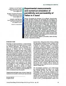
3.4. Computational modeling results Using the computational model described in Section 2.3, we have simulated the fire experiments for a variety of conditions. The experimental runs 2 and 3 are chosen for illustration to further analyze marginal burning condition. The surface area-to-volume ratio is r = 2300 m�1, an averaged value from the samples [20]. The packing ratio is b = 0.01 that was calculated from the fuel loading and the fuel density of qf = 560 kg/m3. The fuel type and packing ratio were equivalent for both runs. The fuel bed depth differed (d = 20 cm for run 2 and d = 40 cm for run 3); fuel loading of run 3 (Fl = 4.2 kg/m2) was double the fuel loading of run 2. Run 2 did not result in fire spread while run 3 did. The time evolution of the calculated pyrolysis gas (CO) contours from ignition to extinction for conditions corresponding to run 2 illustrates fire spread failure (Fig. 3A, d = 20 cm), consistent with the experimental result. The amount of fuel gas due to pyrolysis decreased with time; a successful fire spread would have a constant rate of production of pyrolysis gas after ignition as shown in Fig. 3B (d = 40 cm) for run 3. For the same packing ratio, increasing fuel bed depth or fuel loading will result in an enhanced probability of fire spread success. At this point, the numerical results are in good agreement with the experimental observations. The spread rate approximated from the time evolution of pyrolysis gas is 0.2 m/min, which is in good agreement with the observed experimental fire spread rate of 0.17 m/min. To further understand the relationship of heat transfer and fuel combustion on marginal burning, the time evolution of solid phase temperature, and accumulated heat absorbed by solid particles in a computational cell are illustrated in Fig. 4. It corresponds to a successful fire spread case for d = 40 cm. These heat transfer contributions, Qconv, Qrad, and Qmass, are convective heat flux between the gas phase and the solid, radiative heat flux, and heat release due to water vaporization, pyrolysis, and fuel combustion, respectively. To ignite fuel, a solid particle needs sufficient heat energy. In the preheat region (time from 0 to 26 s), the most effective energy source is radiative heat transfer, Qrad. The solid particle temperature increases but at a relatively low rate. The thermochemical contribution, Qmass, remains negative due to water vaporization. Due to a 20 cm separation distance with the ignition zone, the temperature of gas phase is lower than that of solid phase, which leads to a negative convective heat. When the fire front is close to the observation point, Qrad continues to increase steadily, however, Qconv rises dramatically. This leads to a rapid increase in solid phase temperature from about 450 to 1200 K in a short time. This implies that the fuel particle is ignited. In the ignition zone, due to
X. Zhou et al. / Proceedings of the Combustion Institute 30 (2005) 2287–2294
2293
increase of solid particle, more water is vaporized. There is a sharp decrease in Qmass. After ignition, due to high temperature, the solid phase losses heat by Qrad and Qconv, and solid temperature decreases. On the other hand, due to the heat of char combustion, which compensates for losses from water vaporization and pyrolysis processes, the solid particle temperature remains constant at about 750 K. Analyzing the unsuccessful fire spread case of d = 20 cm results show that there is not enough energy of Qconv and Qrad to compensate the losses of Qmass, especially at the time of ignition. An increase in fuel loading means more energy can be transferred to the unburned region. Similarly, wind and slope enhance Qconv and Qrad, and increase the probability of fuel burning. Conversely, high moisture content stops fuel burning because of the heat loss due to water vaporization. 4. Conclusion
Fig. 3. Time evolution of calculated pyrolysis gas (CO) contours: (A) fuel bed depth is 20 cm, and the fire spread is failure; (B) fuel bed depth is 40 cm and the fire spread is successful, and vectors denote the velocity directions at t = 75 s with a maximum speed of 5 m/s. The rectangular frame denotes the fuel bed.
Current fire spread models do not adequately model the transition between no spread and spread in live fuels. We have conducted 115 experiments to determine the importance of fuel and environmental variables on fire spread success for four different species of chaparral in the laboratory. In examining the applicability of a modified WilsonÕs rule to marginal burning of live chaparral fuel, it was found this rule can give reasonable results for some cases but needs to include more environmental variables. Using a stepwise logistic regression method to analyze these 115 fires, a stepwise logistic regression model was developed to predict the probability of fire spread success. Five variables, viz., wind, slope, dry fuel loading, fuel moisture content, and relative humidity (or environmental temperature), were selected by the model. Analyses indicated the importance of wind speed on fire spread success. The laboratory fires were simulated using a two-dimensional multiphase model. Numerical results are consistent with the experimental observations. The simulated heat transfer processes and combustion mechanism in the fuel bed are helpful for us to understand the factors that determine fire spread success.
Acknowledgments
Fig. 4. Time evolution of solid particle temperature and accumulated heats absorbed by solid particles in a computational grid cell, which is located initially at a distance of 20 cm downwind from the ignition zone.
The funding source for this research is the USDA/USDI National Fire Plan administered through a Research Joint Venture Agreement No. 01-JV-11272166-135 with the Forest Fire Laboratory, Pacific Southwest Research Station, Riverside, CA. We appreciate the efforts of Joey Chong, David Kisor, and Lulu Sun in collecting the fuels, building the fuel beds, and assisting with the experimental burns. S.M. acknowledge partial
2294
X. Zhou et al. / Proceedings of the Combustion Institute 30 (2005) 2287–2294
support from the Wildland Fire R&D Collaboratory, a consortium administered by the National Center for Atmospheric Research.
[10]
References
[11]
[1] P.L. Andrews, BEHAVE Fire Behavior Prediction and Fuel Modeling System, USDA Forest Service Gen. Tech. Rep. INT -194. Ogden, UT, 1986. [2] J.D. Cohen, Estimating Fire Behavior with Forecast: UserÕs Manual. Gen. Tech. Report PSW-90, 1986 May. [3] R.C. Rothermel, A Mathematical Model for Predicting Fire Spread in Wildland Fuels. USDA Forest Service Res. Paper INT -115, Ogden, UT, 1972. [4] S. Raybould, T. Roberts, Fire Manag. Note 44 (4) (1983) 7–10. [5] D. Campbell, The Campbell Prediction System. Wildland Fire Specialists, Ojai, CA 1995. [6] R.C. Rothermel, C.W. Philpot, J. For. 71 (1) (1973) 640–643. [7] F.A. Albini, B.J. Stocks, Combust. Sci. Technol. 48 (1986) 65–76. [8] L.R. Green, Burning by Prescription in Chaparral. USDA Forest Service, Gen. Tech. Rep. PSW-51, 1981. [9] A.D. Bruner, D.A. Klebenow, Predicting Success of Prescribed Fires in Pinyon-Juniper Woodland in
[12] [13] [14] [15] [16] [17] [18] [19] [20]
Nevada. USDA Forest Service Res. Paper INT 219, Ogden, UT, 1979. W.L. McCaw, Predicting Fire Spread in Western Australian Mallee-Heath Shrubland, Ph.D. dissertation, University of New South Wales, Canberra, Australia, 1997. D.R. Weise, G.S. Biging, For. Sci. 43 (2) (1997) 170–180. R.A. Wilson Jr., A Reexamination of Fire Spread in Free Burning Porous Fuel Beds. USDA Forest Service Res. Paper INT -289, Odgen, UT, 1982. R.A. Wilson Jr., Combust. Sci. Technol. 44 (1985) 179–194. X. Zhou, J.C.F. Pereira, Fire Mater. 24 (2000) 37–43. B. Porterie, D. Morvan, J.C. Loraud, M. Larini, Phys. Fluids 12 (7) (2000) 1762–1782. H.R. Baum, O.A. Ezekoye, K.B. McGrattan, R.G. Rehm, Theor. Comput. Fluid Dyn. 6 (1994) 125–139. D.W. Hosmer, S. Lemeshow, Applied Logistic Regression, second ed. Wiley, New York, 2000. B.F. Magnussen, B.H. Hjertager, Proc. Combust. Inst. 16 (1976) 719–729. S.V. Patankar, Numerical Heat Transfer and Fluid Flow, 1980. Hemishpere, New York. C.M. Countryman, C.W. Philpot, Physical Characteristics of Chamise as a Wildland Fuel. USDA Forest Service Res. Paper PSW -66, 1970, Berkeley, CA.
Comment Oleg Korobeinichev, Russian Academy of Sciences, Russia. Could you please comment on whether kinetics and product composition of chaparral fuel pyrolysis were used for modeling of their combustion? Reply. In this paper the numerical model was used primarily as an exploratory tool to analyze the experi-
mental results and gain a better understanding of various heat transfer mechanisms. At the present time there is no accurate model for pyrolysis of chaparral fuel; the kinetic parameters of the rate and product composition are taken from the model of Porterie et al. ([15], in the paper) for pine needles.