A Project on Gesture Recognition with Neural ... - Sven Koenig

A Project on Gesture Recognition with Neural Networks for “Introduction to Artificial Intelligence” Classes Xiaoming Zheng Sven Koenig Department of Computer Science University of Southern California 300 Henry Salvatori Computer Science Center (SAL) 941 W 37th Street Los Angeles, CA 90089-0781 {xiaominz, skoenig}@usc.edu

Abstract This stand-along neural network project for an undergraduate or graduate artificial intelligence class relates to video-game technologies and is part of our effort to use computer games as a motivator in projects without the students having to use game engines. Neural networks are among the most important machine learning techniques and thus good candidates for a project in artificial intelligence. In this project, the students need to understand and extend an existing implementation of the back-propagation algorithm and apply it to recognizing static hand gestures in images. This project requires students to develop a deep understanding of neural networks and the back-propagation algorithm. It extends a project from Tom Mitchell’s “Machine Learning” book and builds on ideas, text and code from that project (courtesy of Tom Mitchell). The project is versatile since it allows for theoretical questions and implementations. We list a variety of possible project choices, including easy and difficult questions.

Introduction The Department of Computer Science at the University of Southern California created a Bachelor’s Program in Computer Science (Games) and a Master’s Program in Computer Science (Game Development), which not only provide students with all the necessary computer science knowledge and skills for working anywhere in industry or pursuing advanced degrees but also enable them to be immediately productive in the game-development industry. They consist of regular computer science classes, game-engineering classes, game-design classes, game cross-disciplinary classes and a final game project. See Zyda and Koenig, Teaching Artificial Intelligence Playfully, Proceedings of the AAAI-08 Education Colloquium, 2008 for more information. The undergraduate and graduate versions of the “Introduction to Artificial Intelligence” class at the University of Southern California are regular computer science classes that are part of this curriculum. We are now slowly converting these classes to use games as the domain for projects because games motivate students, which we believe increases enrollment and retention and helps us to educate better computer scientists. Artificial intelligence becomes more and more important for computer games, now that games use graphics libraries that produce stunning graphics and thus no longer gain much of a competitive 1

advantage via their graphics capabilities. Many games need trajectory-planning capabilities and thus use search algorithms. Some games already use machine learning or planning algorithms. For example, “Black and White” uses a combination of inductive learning of decision trees and reinforcement learning with (artificial) neural networks, and “F.E.A.R” uses goal-oriented action planning. Thus, games can be used to illustrate many areas of artificial intelligence. It was tempting for us to use a publicly available game engine throughout the class and then ask the students to perform several projects in it, such as a search project to plan the trajectories of the game characters and a machine-learning project to make them adapt to the behavior of their opponents. However, students familiar with game development already have plenty of exposure to game engines while students not interested in game development do not need the additional overhead. To put all students on the same footing and allow them to concentrate on the material taught in class, we decided to go with several small projects that do not need large code bases. This technical report describes one particular project from the undergraduate and graduate versions of the “Introduction to Artificial Intelligence” class. Neural networks are among the most important machine learning techniques and thus good candidates for a project in artificial intelligence. We therefore developed a project where the students need to use neural networks to recognize user gestures for computer games. Our goals are two-fold: First, we want students to recognize that neural networks are a powerful and practical techniques for solving complex real-world problems, such as gesture recognition. Second, we want the students to understand both neural networks and the back-propagation algorithm in detail. The students need to understand an existing implementation of the back-propagation algorithm and extend it to answer questions that require computational thinking. Overall, the neural network project is versatile since it allows for theoretical questions and for implementations. We list a variety of possible project choices, including easy and difficult questions. Teachers need to select among them since we list too many of them for a project of a reasonable size and some of them are difficult research questions. (Questions tagged with asterisks are the ones that we tend to use in our own projects.) Teachers also need to provide information on what the students need to submit for their projects (for example, whether they need to submit their programs or the weights of their neural networks after training), how they should submit their projects (for example, on paper or electronically) and by when they need to submit their projects. If you are using this assignment in your class or have any questions, comments or corrections, please send us an email at [email protected]. If you need to cite this assignment (in your own publications or to give us credit), please cite this technical report as Xiaoming Zheng and Sven Koenig, A Project on Gesture Recognition with Neural Networks for Computer Games for “Introduction to Artificial Intelligence” Classes, Technical Report, Department of Computer Science, University of Southern California, Los Angeles (California, USA). Updates, errata and supporting material for the project can be found on our webpages idm-lab.org/gameai, where we will also release additional projects in the future. If there is sufficient interest, we will create sample solutions for teachers at accredited colleges and universities.

Acknowledgments This initiative was partly supported by a grant from the Fund for Innovative Undergraduate Teaching at the University of Southern California. Our project extends a project from Tom Mitchell’s “Machine Learning” book published by McGraw Hill in 1997, namely the project on 2

“Neural Networks and Face Image” (which is available from his website), and builds on ideas, text and code from that project. We thank Tom Mitchell for allowing us to use this material. We also thank Mohit Goenka, Vinay Sanjekar, Qingqing Zuo, Linfeng Zhou, Max Pflueger, Zhiyuan Wang, Aidin Sadighi, Mufaddal Jhaveri, Karun Channa, Abhishek Patnia, Andrew Goodney, Anurag Ojha and all other students who volunteered to provide gesture images and comments.

3

1

Project: Gesture Recognition for Computer Games

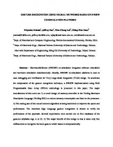
Figure 1: Controlling Games with Gestures (www.engadget.com) The Nintendo Wii is a big success because its motion-sensitive paddle lets users innovatively control objects on the screen with hand gestures. Still, some people say that all gaming instruments that we use today will look ridiculously old-fashioned and redundant in ten years as reported by Matt Marshall in the online document, Gesture Recognition Technology for Games Poised for Breakthrough on the website of VentureBet (http://venturebeat.com/). In the near future, for example, users will likely be able to control objects on the screen with empty hands, as shown in Figure 1. Companies, such as GestureTek (www.gesturetek.com) and Oblong Industries (www.oblong.net), are currently developing the necessary hardware and software to track hands and recognize hand gestures.

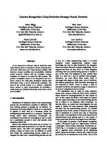
Figure 2: Hand Gestures for the English Alphabet We limit our ambition to a static variant of the gesture recognition problem, where the computer has to classify hand gestures in single images. As an example, Figure 2 presents an image collection of hand gestures for the English alphabet, as given in Dinh, Dang, Duong, Nguyen, Le, Hand Gesture Classification Using Boosted Cascade of Classifiers, Proceedings of the IEEE 2006 International Conference on Research, Innovation and Vision for the Future. After taking some time to understand and memorize these hand gestures, most people are able to recognize 4

them in new images. However, gesture recognition is nontrivial for computers. For example, most people are able to recognize each image in Figure 3 as the hand gesture “thumbs up’ but computers can easily get confused by the different hands, angles, backgrounds, lighting conditions and other differences.1

Figure 3: Different Hand Gestures for “Thumbs Up” In this project, we use (artificial) neural networks to recognize hand gestures in single images. Neural networks are among the most important machine learning techniques. They are too general to reliably classify a large number of hand gestures without any preprocessing of the images but are able to classify a small number of hand gestures out of the box. There exist more specialized gesture recognition techniques that scale much better but the advantage of neural networks is their generality. They are able to solve a large number of classification problems (not just gesture recognition problems), and are thus often ideal solutions for simple classification problems and for prototyping solutions of more complex classification problems.

1.1

Design Decisions for Neural Networks

We make the following design decisions, some of which will be relaxed in the questions: • Topology: We use a one-hidden-layer feedforward neural network, that consists of one layer of hidden units and one layer of output units, as shown in Figure 4. One-hiddenlayer feedforward neural networks are able to represent all continuous functions if they have a sufficiently large number of hidden units and thus are more expressive than single perceptrons. • Activation Function: We use the sigmoid function

σ(x) =

1 1 + e−x

as activation function for all units. The derivative of the sigmoid function is

σ ′ (x) = σ(x)(1 − σ(x)). 1

The second image of Figure 3 was obtained from the website of Istockphoto (www.istockphoto.com), the third image was obtained from the website of Fotolia (www.fotolia.com), and the last image was obtained from the website of Freewebphoto (www.freewebphoto.com).

5

Weights wkj

Weights wji

. . .

Inputs uk

. . .

Hidden units uj

. . .

Output units ui

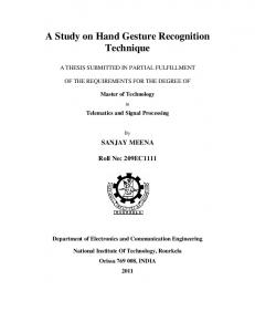
Figure 4: One-Hidden-Layer Feedforward Neural Network • Input Encoding: We subsample the images and then represent them as matrixes of intensity values, one per pixel, ranging from 0 (= black) to 255 (= white). Figure 5 (a) shows the original image of a hand gesture, Figure 5 (b) shows a subsampled image of size 18 × 12, and Figure 5 (c) shows the intensity values of the pixels of the subsampled image. Each intensity value is then linearly scaled to the range from 0 to 1 and becomes one input of the neural network.

(a)

(b)

(c)

Figure 5: Input Encoding • Output Encoding: Each output of the neural network corresponds to a combination of 6

the values of its output units. Imagine that a neural network has to decide whether an image contains the hand gesture “thumbs up.” In this case, we can use one output unit and map all output values greater than 0.5 to “yes” and all output values less than or equal to 0.5 to “no.” • Error Function: We use the sum of squared errors as error functions. Consider a single training example e, where ti [e] represents the desired output and oi the actual output of output unit ui . Then, the difference of the desired and actual output is calculated as

E[e] =

1.2

1X (ti [e] − oi )2 . 2 i

The Back-Propagation Algorithm

1 procedure back-propagation(trainingset, neuralnetwork, α) 2 inputs 3 trainingset: the training examples, each specified by the inputs xk [e] and desired outputs ti [e]; 4 neuralnetwork: a one-hidden-layer feedforward neural network with weights wkj and wji 5 α: the learning rate 6 repeat 7 for each e in trainingset do 8 /* propagate the input forward */ 9 for eachP hidden unit uj do w x [e] 10 aj := k kj k 11 oj := 1/(1 + e−aj ) 12 for eachP output unit ui do 13 ai := w o j ji j

14 oi := 1/(1 + e−ai ) 15 /* propagate the error backward */ 16 for each output unit ui do 17 δi := oi (1 − oi )(ti [e] − oi ) 18 for each hidden unit uj do 19 wji := wji + α · δi · oj 20 for each hidden unit P uj do 21 δj := oj (1 − oj ) i wji δi 22 for each input unit uk do 23 wkj := wkj + α · δj · xk [e] 24 until the termination condition is satisfied

Figure 6: Back-Propagation Algorithm The pseudocode of the back-propagation algorithm repeatedly iterates over all training examples, as shown Figure 6. Each iteration is called an epoch. For each training example e, it executes two parts of code. The first part of the code propagates the inputs forward through the neural network to calculate the outputs of all units [Lines 8-14]. Line 10 calculates the weighted sum aj of the inputs of a hidden unit uj from the inputs xk [e] of the neural network. Line 11 calculates the output oj of the hidden unit by applying the sigmoid function to the weighted sum ai of its inputs. Similarly, Line 13 calculates the weighted sum of the inputs of an output unit ui from the outputs oj of the hidden units. Line 14 calculates the output oi of the hidden unit (which is an output of the neural network) by applying the sigmoid function to the weighted sum of its inputs. The second part of the code propagates the error backward through the neural network and updates the weights of all units using gradient descent with a user-provided learning rate α [Lines 15-23], which is typically a small positive constant close to zero. The available examples are usually partitioned into the training examples and the cross validation examples, and the back-propagation algorithm terminates once the error over all cross validation

7

examples increases (to prevent overtraining), where the error of a set of examples is the average of the errors of the examples contained in the set. We now derive the update rule for the weights wji of the output units. The update rule of the weights wkj of the hidden units is similar. The weights wji of output unit ui are updated using gradient descent with learning rate α, that is, changed by a small step against the direction of the gradient of the error function to decrease the error E[e] quickly:

wji := wji − α · The input of unit ui is ai =

P

j

∂E[e] . ∂wji

wji oj [Line 13], resulting in

∂E[e] ∂E[e] ∂ai ∂E[e] ∂E[e] ∂oi = · = · oj = · · oj . ∂wji ∂ai ∂wji ∂ai ∂oi ∂ai The error is E[e] =

1 2

P

i (ti [e]

− oi )2 , resulting in

∂E[e] ∂ 1 = (ti [e] − oi )2 = −(ti [e] − oi ). ∂oi ∂oi 2 The output of unit ui is oi = σ(ai ) [Line 14], resulting in

∂oi = σ(ai )(1 − σ(ai )) = oi (1 − oi ). ∂ai Thus, the update rule for the weights wji [Line 19] is

∂E[e] ∂wji := wji − α(−(ti [e] − oi )oi (1 − oi )oj )

wji := wji − α · wji

wji := wji + α(ti [e] − oi )oi (1 − oi )oj wji := wji + αδi oj , where we define δi = (ti [e] − oi )oi (1 − oi ) for simplification.

1.3

gesturetrain

You will use gesturetrain, which is a modified version of a program by Tom Mitchell and his students from Carnegie Mellon University. The next two sections contain modified descriptions of that program. We thank Tom Mitchell for allowing us to use this material.

8

1.3.1

Running gesturetrain

gesturetrain has several options that can be specified on the command line. A short summary of these options can be obtained by running gesturetrain with no arguments. -n - This option either loads an existing network file or creates a new one with the given filename. The neural network is saved to this file at the end of training. -e - This option specifies the number of epochs for training. The default is 100. -T - This option suppresses training but reports the performance for each of the three sets of examples. The misclassified images are listed along with the corresponding output values. -s - This option sets the seed for the random number generator. The default seed is 102194. This option allows you to reproduce experiments, if necessary, by generating the same sequence of random numbers. It also allows you to try a different sequence of random numbers by changing the seed. -S - This option specifies the number of epochs between saves. The default is 100, which means that the network is only saved at the end of training if you train the network for 100 epochs (also the default). -t - This option specifies the filename of a text file that contains a list of image pathnames, one per line, that is used as training set. If this option is not specified, training is suppressed. The statistics for this set of examples is all zeros but the performance is reported for the other sets of examples. -1 - this option specifies the filename of a text file that contains a list of image pathnames, one per line, that is used as non-training set (typically the cross validation set). If this option is not specified, the statistics for this set of examples is all zeros. -2 - this option specifies the filename of a text file that contains a list of image pathnames, one per line, that is used as non-training set (typically the test set). If this option is not specified, the statistics for this set of examples is all zeros. 1.3.2

Output of gesturetrain

gesturetrain first reads all data files and prints several lines about these operations. It then begins training and reports the performance on the training, cross validation and test sets on one line per epoch: These values have the following meanings: epoch is the number of epochs completed (zero means no training has taken place so far). delta is the sum of all δ values of the hidden and output units over all training examples. trainperf is the percentage of training examples that were correctly classified. 9

trainerr is the average of the errors of all training examples. test1perf is the percentage of cross validation examples that were correctly classified. test1err is the average of the errors of all cross validation examples. test2perf is the percentage of test examples that were correctly classified. test2err is the average of the errors of all test examples. 1.3.3

Implementation of gesturetrain

The code of gesturetrain is broken into several modules: • gesturetrain.c is the top-level program that uses all of the modules below to implement the gesture recognition. You might have to set the size of the neural network and the training parameters in this module, both of which are trivial changes. You might also have to modify both performance on imagelist and evaluate performance to change the performance evaluation. • backprop.c and backprop.h are the neural network module, that provides high level routines for creating, training and using neutral networks. You might have to understand all of the code in this module to answer some of the questions. • imagenet.c is the interface module, that generates the inputs of a neural network from images and sets the desired outputs for training. You might have to modify load target when changing the output encoding. • hidtopgm.c is the hidden unit weight visualization module. You do not have to modify anything in this module, although it may be interesting to explore some of the numerous possible alternative visualization schemes. • pgmimage.c and pgmimage.h are the image module, that provides the ability to read and write PGM image files and to read and write image pixels. You do not have to modify anything in this module. We now describe the code of the neural network module in more detail. We begin with a brief description of its data structure, a Back Propagation Neural Network BPNN. All unit values and weight values are stored as doubles in a BPNN. The inputs, hidden units and output units are indexed starting at 1. You can get the number of inputs, hidden units and output units of a BPNN *net with net->input n, net->hidden n and net->output n, respectively. You can get the value of the kth input, hidden unit and output unit (= actual output) with net->input units[k], net->hidden units[k] and net->output units[k], respectively. You can get the desired output with net->target[k]. You can get the value of the weight that connects the ith input unit to the jth hidden unit with net->input weights[i][j]. Similarly, you can get the value of the weight that connects the jth hidden unit to the kth output unit with net->hidden weights[j][k]. The routines are as follows:

10

void bpnn initialize(seed) int seed; This routine initializes the neural network package. It should be called before any other routines in the package are used. Currently, it only initializes the random number generator with the given seed. BPNN *bpnn create(n in, n hidden, n out) int n in, n hidden, n out; This routine creates a new BPNN with n in inputs, n hidden hidden units and n output output units. All weights are randomly initialized to values in the range from -1.0 to 1,0. The routine returns a pointer to a BPNN or, in case of failure, NULL. void bpnn free(net) BPNN *net; This routine frees all memory associated with a BPNN. void bpnn train(net, learning rate, momentum, erro, errh) BPNN *net; double learning rate, momentum; double *erro, *errh; This routine runs the back-propagation algorithm on a BPNN. It assumes that the inputs and desired outputs have been properly set up. learning rate and momentum need to be values in the range from 0.0 to 1.0. errh and erro are pointers to doubles, which are set to the sum of all δ values of the hidden and output units, respectively, over all training examples. void bpnn feedforward(net) BPNN *net; This routine determines the actual output values for the input values of a BPNN. BPNN *bpnn read(filename) char *filename; This routine allocates memory for a BPNN, initializes it with the weights stored in the network file with a given filename and returns a pointer to this new BPNN or, in case of failure, NULL. void bpnn save(net, filename) BPNN *net; char *filename; This routine saves a given BPNN to a file with a given filename.

2

Questions

Answer the following questions.

11

Question 1: Very Difficult We derived the update rule for the weights wji of the output units ui earlier in the project text. Show that the update rule of the weights wkj of the hidden units uj under the same assumptions is

wkj := wkj + α · oj (1 − oj )

X

(wji δi ) · xk [e],

i

as shown on Lines 21 and 23 in the pseudocode of the back-propagation algorithm from Figure 6. Justify all steps of the derivation. (Hint: Your artificial intelligence textbook is likely to explain the derivation.)

* Question 2: Moderately Difficult Derive the update rule for the weights wji of the output units ui and the weights wkj of the hidden units uj if the tanh function

tanh(x) =

ex − e−x ex + e−x

is the activation function of all units instead of the sigmoid function. The derivative of the tanh function is

tanh′ (x) = 1 − tanh2 (x). Justify all steps of the derivation. Explain why it is reasonable to consider the tanh function as activation function.

Question 3: Easy Describe the purpose of each statement of function bpnn train in file backprop.c and list the corresponding line(s), if any, in the pseudocode of the back-propagation algorithm from Figure 6.

* Question 4: Moderately Difficult Understand how the code of function bpnn adjust weights updates the weights of all units. Assume that the values of the weights wji of the output units ui and the weights wkj of the t and w t , respectively. Using this hidden units uj at the current time t are denoted by wji kj notation, formally express the update rules for the weights of the output and hidden units for the next training example as implemented in the code, explain the main difference between the update rules used in the code and the ones given earlier in the project text and describe the advantage of the update rules used in the code. 12

* Question 5: Easy Train a neural network using the default training parameter settings (learning rate 0.3 and momentum 0.3) for 75 epochs, by deleting the file “gesture.net” (a previously built neural net) to train the neural network from scratch and then using the following command to create and train the neural network: gesturetrain -n gesture.net -t downgesture train.list -1 downgesture test1.list -2 downgesture test2.list -e 75 The 156 images are split randomly into the test set that contains roughly 1/3 (= 52) of the examples. The test examples are stored in downgesture test2.list and are used to evaluate the error of the neural network after training. Test examples are typically unnecessary during training. We need them in this project to determine the error of the neural network on unseen examples after training. The remaining examples are used for training. They are split randomly into a training set that contains roughly 2/3 (= 70) of the remaining examples and a cross validation set that contains roughly 1/3 (= 34) of the remaining examples. The training examples are stored in downgesture train.list and are used by the update rule to adjust the weights of all units. The cross validation examples are stored in downgesture test1.list and are used to terminate training once the error over them increases. gesture.net contains the neural network after training. Explain why the backpropagation algorithm uses a training and a cross validation set and terminates once the error over all cross validation examples (instead of, say, all training examples) increases. Read Section 1.3.2 carefully. Then, graph the error on the training set, cross validation set and test set as a function of the number of epochs. Explain your experimental results (including your observations, detailed explanations of the observations and your overall conclusions).

* Question 6: Easy Repeat the experiment from Question 5 but stop training after the epoch when the error on the cross validation set is minimal. Then, examine the weights of the hidden units of the resulting neural network as follows: Type make hidtopgm to compile the utility on your system. Type hidtopgm gesture.net image-filename 32 30 n to create a visualization of the weights of hidden unit n in image-filename, that can be displayed with image display programs such as xv. The lowest weights are mapped to pixel value 0, and the highest weights are mapped to pixel value 255. Explain whether the hidden units seem to weight some regions of the images more than others and whether different hidden units seem to be tuned to different features of some sort. If the visualizations look like noise, type make gesturetrain init0 and then use gesturetrain init0 instead of gesturetrain, which initializes the weights of the hidden units before training to zero rather than random values.

* Question 7: Moderately Difficult Think about how to change the given code to classify four hand gestures, namely “up,” “down,” “hold” and “stop.” Try at least two different output encodings. For each output encoding, describe the output encoding, change the code appropriately, explain your code changes and 13

experimentally determine the error on the test set as in Question 5 except that you stop training after the epoch when the error on the cross validation set is minimal and then report the error on the test set. Compare the experimental results for both output encodings (including your observations, detailed explanations of the observations and your overall conclusions). (Hint: You could try a neural network with one output whose value is split into four ranges, one for each hand gesture. You could try a neural network with two outputs, that encode the hand gesture in binary. You could also try a neural network with four outputs, one for each hand gesture.)

* Question 8: Moderately Difficult Change the given code to implement the update rule for the weights that you derived in Question 2. Answer Question 5 both for the old and new code and compare the experimental results (including your observations, detailed explanations of the observations and your overall conclusions).

Extra Credit 1: Open Ended We have assumed so far that the hand gestures fill the whole image. Often, however, hand gestures will only be part of the image and the size of the hand will vary from image to image. Extend the given code to find all instances of the hand gesture “thumbs up” in a given image, similar to modern cameras that are able to find all faces in the current camera image, no matter what their sizes are.

Extra Credit 2: Open Ended We have assumed so far that the hand gestures are static, that is, involve stationary hands. Often, however, hand gestures will be dynamic, that is, involve moving hands. Extend the given code to recognize several simple dynamic hand gestures. Your approach could be simple (for example, use Bobick and Davis, The Representation and Recognition of Action Using Temporal Templates, IEEE Transactions on Pattern Analysis and Machine Intelligence, 23(3), 2001, pages 257-267 as inspiration) or as complex as you like.

14