Appl. Math. Inf. Sci. 6, No. 3, 515-524 (2012)
515
Applied Mathematics & Information Sciences An International Journal c 2012 NSP ° Natural Sciences Publishing Cor.
A Projected Gradient Method for a High-order Model in Image Restoration Problems Zhi-Feng Pang1 , Baoli Shi1 and Lihong Huang2,3 1
College of Mathematics and Information Science, Henan University, Kaifeng, 475004, China College of Mathematics and Econometrics, Hunan University, Changsha, 410082, China 3 Hunan Women’s University, Changsha, 410004, China 2
Received: Sep 3, 2011; Revised Oct. 4, 2011; Accepted May. 11, 2012 Published online: 1 Sep. 2012
Abstract: Based on the augmented Lagrangian strategy, we propose a projected gradient method for solving the high-order model in image restoration problems. Based on the Berm`udez and Moreno (BM) algorithm, the convergence of the proposed method is proved. We also give the relationship that the semi-implicit gradient descent method can be deduced from the projected gradient method. Some numerical experiments are arranged to demonstrate the efficiency of the proposed method for restoring the gray-level and color images. Keywords: Augmented Lagrangian strategy, high-order model, Kronecker product, projected gradient method, semi-implicit gradient descent method.
1. Introduction During the past two decades, the restoration of digital images based on variational models and optimization techniques has been extensively studied in many areas of image processing and computer vision such as image denoising, image deblurring, image zooming and image inpainting, etc. [1, 9]. Among these variational models, a frequently used model proposed by Rudin, Osher, and Fatemi (ROF) [19] considers to solve the following problem Z α (f − u)2 dx + |u|BV (Ω) , min (1) u 2 Ω where Ω ⊂ R2 with Lipschitz boundary, BV (Ω) is the space of functionals with bounded variation and α is the regularization parameter. Since the ROF model has the ability to preserve image edges, this model and its variants have been widely used in the image restoration problems [1,9, 18]. However, in the course of restoring the deteriorated image, the ROF model is well known to make the solution be piecewise constant (called the staircasing effect). To overcome this effect, some high-order PDEs [5, 10, 17, 21, 25] have been introduced. Its reason is that the high∗
order PDEs can damp the oscillations much faster and require much stronger smoothness. One of high-order PDEs has been proposed by Lysaker, Lundervold, and Tai [17] as follows: Z λ min (f − u)2 dx + |u|BV 2 (Ω) , (2) u 2 Ω where λ is the regularization parameter and BV 2 (Ω) called the second-order bounded variation space is defined by nZ |u|BV 2 (Ω) = sup udiv2 ξdx|ξ ∈ Cc2 (Ω), Ω o kξkL∞ (Ω) ≤ 1 < ∞. In when u ∈ W 2,1 (Ω), we can get |u|BV 2 (Ω) = R fact, 2 |∇ u|dx, where ∇2 u denotes the Hessian of u. ObviΩ ously, we can extend the model (2) to a general high-order model as Z γ min (f − Ku)2 dx + |u|BV 2 (Ω) , (3) u 2 Ω\D where γ is the regularization parameter and D ⊆ Ω. It is obvious that the model (3) is the deblurring problem when K is the convolution operator and D = ∅ [24]. When K
Corresponding author:
[email protected]. c 2012 NSP ° Natural Sciences Publishing Cor.
516
is the identity operator and D 6= ∅, this model turns to the image zooming or inpainting problem [12]. From the numerical point of view, the high-order model similar to the ROF model is not straightforward to be minimized, which is due to the fact that |u|BV 2 (Ω) is not differentiable. Thus a regularization q approach is devised by emR 2 ploying Ω |∇ u|ε dx = u2xx + u2xy + u2yx + u2yy + εdx for a small positive ε to replace |u|BV 2 (Ω) . Following this regularization, an artificial time marching algorithm [17, 26] or a fixed point iteration [22] is used to compute the related solution. But both of these methods suffer from some difficulties such as choosing the suitable parameter ε. On the other hand, it is obvious that the solution obtained by these two methods is not the true solution of the high-order model (3). Another approaches, which can avoid dealing with the nondifferentiable term |u|BV 2 (Ω) , follow from the motivation of Chambolle’s work [6]. These methods use the Legendre-Fenchel transformation to transform the original problem into the related dual problem so that we can easily obtain the solution of the original problem [8, 21,20]. The augmented Lagrangian strategy, which can efficiently combine the advantages of the Lagrangian method and the penalty method, has been successfully applied to the image processing problem [14–16, 23, 24]. Recently, different from the methods by solving some subproblems to find the saddle point of the Lagrangian functions [16, 23,24], Ito and Kunisch in their papers [14, 15] designed a smoothing function to approximate the original nonsmooth function in Hilbert space and then obtained the related solution based on an active set method. Motivated by the work of Ito and Kunisch [14, 15], in this paper, we propose a projected gradient method as a basic method to solve the high-order model (2). This projected gradient method requires a relatively small memory footprint and is easier to solve the high-order model (2) than the active set method used in [14, 15]. Thanks to the Berm`udez and Moreno(BM) algorithm [3], the convergence of the proposed algorithms is proved. We also give the relationship that the typical semi-implicit gradient descent algorithm [8] can be naturally deduce from this projected gradient method. Furthermore, different from the augmented Lagrangian method used to solve the image deblurring problem [24] and the artificial time marching method to solve image zooming [14] or the image inpainting problem[12], we also extend to this projected gradient method to efficiently solve these aforementioned image restoration problems. The plan of the paper is as follows. We first recall some results about the augmented Lagrangian strategy in Section 2. Then we propose a projected gradient method to solve the high-order model based on the augmented lagrangian strategy and give the convergence result of this method in Section 3. Furthermore, we also refer to the relationship between the projected gradient method and the typical semi-implicit gradient descent method in this section. We present experimental results in support of our pro-
c 2012 NSP ° Natural Sciences Publishing Cor.
Zhi-Feng Pang: et al : A Projected Gradient Method ...
posed algorithms in Section 4, followed by some conclusions in Section 5.
2. Augmented Lagrangian method Augmented Lagrangian method has many advantages over the Lagrangian method and the penalty method, which was recently applied to solve nonsmooth, convex optimization problems in image processing [14–16,23,24]. However, different from its applications in [16,23,24], Ito and Kunisch [14,15] proposed a Lagrangian smoothing regularization strategy in Hilbert space, which gives us equivalent but regularized strategy. Now, we recall this strategy and give some related results. Set X, Y be Hilbert spaces. Assume that g : X → R is a continuously differentiable, convex function and ϕ : Y → R is a proper, lower semicontinuous, convex function. Furthermore, we also assume that ϕ is nondifferentiable in origin and X = X ∗ . Let us consider the following optimization problem min g(u) + ϕ(Λu), (4) u∈X
where Λ : X → Y is a bounded linear operator. Then, based on the results [11], the following statement holds. Lemma 1.The necessary and sufficient condition for u∗ ∈ X to be the minimizer of (4) is given by ½ ∗ ξ ∈ ∂ϕ(Λu∗ ), (5) g 0 (u∗ ) + Λ∗ ξ ∗ = 0, where ∂ϕ(x) denotes the subdifferentiable at the point x [11] which is defined by ∂ϕ(x) = {x∗ ∈ X : ϕ(y) − ϕ(x) ≥ (x∗ , y − x) ∀y ∈ X}. It is obvious that u∗ satisfying (5) implies that u∗ is the solution of (4). However, due to the nondifferentiable of ϕ, it is difficult to find some efficiently numerical methods to obtain it. To overcome this drawback, a regularization method [14,15] was proposed by designing a smooth approximation based on the augmented Lagrangian strategy. That is to say, we can equivalently convert the problem (4) into the following constrained problem ½ min g(u) + ϕ(Λu − v), (6) subject to v = 0 in X. The equality constraint v = 0 in (6) can be treated by the augmented Lagrangian method. By employing the augmented Lagrangian strategy [13], we can transform the constrained optimization problem (6) into the following unconstrained problem c min g(u) + ϕ(Λu − v) + (ξ, v) + |v|2X , (7) 2 where ξ ∈ X is a multiplier and c is a positive penalty parameter. Let n o c ϕc (Λu, ξ) = inf ϕ(Λu − v) + (ξ, v) + |v|2X , (8) v∈X 2 then ϕc (Λu, ξ) is a C 1 approximation of ϕ [14,15].
Appl. Math. Inf. Sci. 6, No. 3, 515-524 (2012) / www.naturalspublishing.com/Journals.asp
Definition 1.Let G : X → R ∪ {∞} be a proper, convex function, then the conjugate function of G is defined by n o G∗ (x∗ ) = sup (x, x∗ ) − G(x) for x∗ ∈ X. x∈X
Lemma 2.The infimum problem (8) can be rewritten as n o 1 ϕc (Λu, ξ) = sup (Λu, y ∗ ) − ϕ∗ (y ∗ ) − |y ∗ − ξ|2 (9) . 2c y ∗ ∈X Furthermore, the supremum of (9) is attained at a unique point ξc (u, ξ) = ϕ0 (Λu, ξ) = Hc (Λu + c−1 ξ). where Hc = c(I − J1/c ). If set δC ∗ (y ∗ ) denote the characteristic function of a closed convex set C ∗ ⊂ X, i.e., δC ∗ (y ∗ ) = 0 if y ∗ ∈ C ∗ , else δC ∗ (y ∗ ) = ∞. Then, for the supremum problem (9), we have the following assertions [14,15]. Lemma 3.Assume that ϕ∗ (y ∗ ) = δC ∗ (y ∗ ) in the supremum problem (9), we have the following assertions: (1)The supremum of (9) is attained at a unique point ξc (u, ξ) = PC ∗ (ξ + cΛu), where PC ∗ (u) denotes the projection of u ∈ X onto C ∗. (2)If ξ ∈ ∂ϕ(Λu) for ξ, u ∈ X, then ξ=PC ∗ (ξ + cΛu) for all c > 0.
3. Projected gradient method To overcome the nonsmoothness of the high-order model (2), some numerical methods have been proposed in [8, 17,21,26,22]. In this section, based on the augmented Lagrangian strategy, we first propose a projected gradient method to solve the high-order model (2) and give the convergence analysis by using the results of the Berm`udez and Moreno(BM) algorithm [3]. Then we arrange some implementation details for the proposed method and also mention that the typical semi-implicit gradient descent algorithm [8] can be deduced from the projected gradient method.
3.1. Projected gradient method for the high-order model R
Set g(u) = λ2 kf − uk2L2 (Ω) , ϕ(Λu) = Ω |Λu|dx and Λ = ∇2 . If assume that u is in the Hilbert space, then the high-order model (2) can be rewritten as a special form of the minimization problem (4). Following from Lemma2.4, we then have the following result.
517
Theorem 1.The solution u∗ of the high-order model (2) satisfies u∗ = f − 1 div2 ξ ∗ , (10a) λ ∗ ξ = PC ∗ (ξ ∗ + c∇2 u∗ ), (10b) where C ∗ is given by C ∗ = {y ∈ X : |y| ≤ 1 a.e. in Ω}. It is not difficult to find that Theorem 3.1 implies the optimality condition of the high-order model (2). Especially, Eq. (10a) is based on the fact that the conjugate function of ϕ(Λu) is a characteristic function on the closed and convex set C ∗ . If we define the following Lagrangian functional Z λ Lc (u, ξ) = (f − u)2 dx + ϕc (∇2 u, ξ), (11) 2 Ω where the definition of ϕc (∇2 u, ξ) is similar to (8), we can deduce that (u∗ , ξ ∗ ) is the saddle point of the Lagrangian functional (11). To get this optimal point (u∗ , ξ ∗ ), we propose the following iterative method. •Algorithm 3.1. Projected Gradient Method. (I)Set ξ 0 = 0 and c > 0; (II)Compute (un , ξ n+1 ) by ½ n u = f − λ1 div2 ξ n , ξ n+1 = PC ∗ (ξ n + c∇2 un ); (III)If the stop criterion is not satisfied, set n := n + 1 and go to step (II). In order to get the convergence result of Algorithm 3.1, we need to recall some results of the Berm`udez and Moreno(BM) algorithm [3]. Assume that V and E are the Hilbert spaces, B : E → V is a bounded linear operator and B ∗ is the adjoint operator of B. With choosing an arbitrarily original value v 0 , the BM algorithm then employs the iterative strategy ½ n v = A−1 (h − By n ), (12) y n+1 = Hη (B ∗ v n + ηy n ) to solve the minimization problem 1 min (Av, v) − (h, v) + φ(v), v∈V 2
(13)
where φ = ψ ◦ B ∗ and ψ : E → R. Berm`udez and Moreno(BM) [2, 3] gave the following convergence result of the algorithm (12). Theorem 2.If the following assumptions hold: (1)A is a linear symmetric coercive operator: (Av, v)V ≥ αkvk2V and is continuous on the finite dimensional subspaces of V ; 0 )+φ(v) → (2)There exists v0 in dom(φ) satisfying (Av,v−v kvk +∞ if kvk → +∞.
c 2012 NSP ° Natural Sciences Publishing Cor.
518
Zhi-Feng Pang: et al : A Projected Gradient Method ...
(3)The parameter η satisfies 0≤η≤
projection of x on the closed convex set C := {y : |y| ≤ 1} can be written as x PC (x) = . max{1, |x|}
2α . kB ∗ k2
where kB ∗ k denotes the L2 norm of the operator B ∗ .
By the above facts, Theorem 3.1 can be reformulated as Then the sequence {v } generated by (12) satisfies lim v = the discrete form below. n
n
n→∞
v ∗ , here v ∗ is the solution of (13). Furthermore, y n * y in E with y ∈ ∂ψ(B ∗ v). If set V = L2 (Ω), E = (L2 (Ω))4 , B = ∇2 , A = λI and h = λf , then all of the assumptions in Theorem 3.2 are satisfied for the high-order model (2). This implies that Algorithm 3.1 is a special case of the BM algorithm. So we get the following result based on Theorem 3.1 and 3.2.
Theorem 3.The solution u∗ of (14) satisfies the following equation 1 T ∗ ∗ (16a) u = f − (M ξ ), λ ∗ ∗ ξ + τ (M u ) . (16b) ξ∗ = max(1, |ξ ∗ + τ (M u∗ )|)
Corollary 1.If the parameter c satisfies
for each τ > 0.
0≤c≤
2λ , k∇2 k2
where k∇2 k denotes the L2 norm of the Hessian operator ∇2 . Then the sequence {un } generated by Algorithm 3.1 converges to the unique solution u∗ of the high-order model (2).
3.2. Projected gradient method and semi-implicit gradient descent method We start by giving a discrete algorithm for solving the high-order model (2). For convenience, we first consider the gray-level image. Let an N × N image be denoted by 2 u ∈ RN with the column lexicographical ordering. Denote the first-order forward difference matrix as D0 , then backward difference matrix can be denoted as −D0T . Assume that u satisfies the zero Neumann boundary condition, then the discretization of (2) can be written as
Then the discretization of Algorithm 3.1 can be rewritten as the following strategy. •Algorithm 3.2. Projected Gradient Method(PGM). (I)Set ξ 0 = 0 and τ > 0; (II)Compute (un , ξ n+1 ) by ( n u = f − λ1 (M T ξ n ), ξ n +τ (M un ) ξ n+1 = max(1,|ξ n +τ (M un )|) ; (III)If the stop criterion is not satisfied, set n := n + 1 and go to step (II). In fact, Algorithm 3.2 is convergent when the parameter τ satisfies some conditions which are based on the spectral radius of M . For the Kronecker product, we recall some of its basic properties if the related matrices are assumed as the N −order real-value square matrices. Lemma 4.For matrices A, B, C and D, the following assertions hold [27]: (1)(A ⊗ B)(C ⊗ D) = (AC) ⊗ (BD). (2)(A ⊗ B)T = AT ⊗ B T , here T denotes the conjugate transpose of the matrix. (3)A ⊗ B is unitary if A and B are unitary. (4)Let σi and µi , i = 1, · · ·N , are the eigenvalues of A and B respectively. Then the eigenvalues of A ⊗ B are
λ min kf − uk2`2 (Ω) + |M u|`1 (Ω) , (14) u 2 where (I ⊗ D0T )(I ⊗ D0 ) I ⊗ (D0T D0 ) (I ⊗ DT )(D0 ⊗ I) DT ⊗ D0 0 0 M = (D0 ⊗ I)(I ⊗ D0T ) = D0 ⊗ D0T (15) (D0T ⊗ I)(D0 ⊗ I) (D0T D0 ) ⊗ I0
Lemma 5.For the matrix A, there exists N −order unitary matrices U and V such that
and |M u|1 is given by
A = U diag(si )V,
N q X 2
|M u|1 =
[M1 u]2i + [M2 u]2i + [M3 u]2i + [M4 u]2i .
i=1
where M1 = I ⊗ (D0T D0 ), M2 = D0T ⊗ D0 , M3 = D0 ⊗ D0T and M4 = (D0T D0 ) ⊗ I and I denotes the N −order identity matrix. Here ⊗ denotes the Kronecker product. Based on the fact that (div2 u, w)X = (u, ∇2 w)Y , it is easy to denote the discrete form of div2 . Furthermore, the
c 2012 NSP ° Natural Sciences Publishing Cor.
σi µi , i = 1, · · ·N.
where diag(si ) is a N −order diagonal matrix with (i, i) entries the singular values of A. Theorem 4.The spectral radius of M satisfies ρ(M ) ≤ 8. Proof.Set S = D0T D0 . By Lemma 3.1, we can deduce that S has the singular value decomposition S = U diag(σi2 )V , here σi is the singular value of D0 , U and V are N −order unitary matrices.
Appl. Math. Inf. Sci. 6, No. 3, 515-524 (2012) / www.naturalspublishing.com/Journals.asp
We notice that D0 is a sparse matrix with 1 and −1 as the only two nonzero elements per row, it is not difficult to deduce that kD0 k∞ = 2. On the other hand, since the largest eigenvalue of M T M is the `2 norm of M , we consider the following matrix: M T M = (I ⊗ S)T (I ⊗ S) + (S ⊗ I)T (S ⊗ I) + (D0T ⊗D0 )T (D0T ⊗ D0 ) + (D0 ⊗ D0T )T (D0 ⊗ D0T ) = I ⊗ (S T S) + (S T S) ⊗ I + (D0 ⊗ D0T )(D0T ⊗ D0 ) + (D0T ⊗ D0 )(D0 ⊗ D0T ) = I ⊗ (S T S) + (S T S) ⊗ I + S T ⊗ S + S ⊗ S T = (V T V ) ⊗ (V T diag(σi4 )V ) + (V T diag(σi4 )V ) ⊗(V T V ) + (V T diag(σi2 )U T ) ⊗ (U diag(σi2 )V ) +(U diag(σi2 )V ) ⊗ (V T diag(σi2 )U T ) = (V T V ) ⊗ (V T diag(σi4 )V ) + (V T diag(σi4 )V ) ⊗(V T V ) + (V T diag(σi2 )U T ) ⊗ (U diag(σi2 )V ) +(U diag(σi2 )V ) ⊗ (V T diag(σi2 )U T ) = (V ⊗ V )T [I ⊗ diag(σi4 ) + diag(σi4 ) ⊗ I](V ⊗ V ) + (V ⊗ U )T [diag(σi2 ) ⊗ diag(σi2 )](V ⊗ U ) +(V ⊗ U )[diag(σi2 ) ⊗ diag(σi2 )](V ⊗ U )T . It is easy to find that the matrices included in [·] of the last equation of M T M are diagonal. Then, with the help of Lemma 3.1, we can deduce that the `2 norm σmax (M T M ) of M satisfies σmax (M T M ) = 2σmax diag(σi4 ) + 2σmax (diag(σi2 ) ⊗diag(σi2 )) = 4||D0 ||42 ≤ 4kD0 k4∞ = 64. Therefore, we have ρ(M ) ≤ 8. 1 Theorem 5.Set τ = λc . Assume that 0 ≤ τ ≤ 32 , then the n sequence {u } generated by Algorithm 2 converges to the solution u∗ of (13).
Proof.With the help of λmax (M T M ) < 64 and Corollary 3.1, it is easy to deduce the assertion. Now we consider the relationship between Algorithm 3.2 and semi-implicit gradient descent method [8]. Actually, Eq. (16b) can be equivalently viewed as ξi∗ (M u∗ )i = |(M u∗ )i | and |ξi∗ | ≤ 1, for all i
(17)
and ξi∗ =
(M u∗ )i if |(M u∗ )i | 6= 0. |(M u∗ )i |
(18)
By the fact that ξi∗ (M u∗ )i ≤ |ξi ||(M u∗ )i | and |ξi∗ | ≤ 1, (17) and (18) can be obviously summarized to ξi∗ |(M u∗ )i | = (M u∗ )i . Hence, (16) can be written as ½ ∗ ui = fi − λ1 (M T ξ ∗ )i , ξi∗ |(M u∗ )i | = (M u∗ )i
(19)
519
for i = 1, 2, · · · N 2 . We then can get ¯³ ´¯ ³ ´ ¯ ¯ ξi∗ ¯ λM f − (M M T ξ ∗ ) ¯ = λM f − (M M T ξ ∗ ) , i
i
which can be solved by semi-implicit gradient descent (or fixed point) method [8] as follows ³³ ´ ξin+1 = ξin + β λM f − (M M T ξ n ) − ¯³ ´¯ i´ ¯ ¯ T n ¯ λM f − (M M ξ ) ¯ξin+1 . i
So we have the following algorithm to solve the problem (2). •Algorithm 3.3. Semi-implicit Gradient Descent Method (SGDM). (I)Set ξ 0 = 0 and γ > 0; (II)Compute (un , ξ n+1 ) by ( n u = f − λ1 (M T ξ n ), ξin +β(λM f −(M M T ξ n ))i ξin+1 = 1+β|(λM ; f −(M M T ξ n ))i | (III)If the stop criterion is not satisfied, set n := n + 1 and go to step (II). 1 Theorem 6.Assume that 0 ≤ γ ≤ 64 . Then the sequence n {u } generated by Algorithm 3.3 converges to the solution u∗ of (14).
Remark.Following from the work in [8] and using the fact that ρ(M ) ≤ 8, it is easy to deduce that the above assertion holds. Actually, Algorithm 3.2 can be viewed as a modified form of Algorithm 3.3 [13, 2]. But here we show that Algorithm 3.3 can be naturally deduced from Algorithm 3.2. Remark.For the color image restoration problems, we can 2 denote that u ∈ R3N . Then the Hessian matrix can be written as M = (Mr ; Mg ; Mb ), here Mj = M given in (15) for j = r, g, b. In this case, the minimization problem (14) can be transformed into the following form λ min kf − uk2`2 (Ω) + |Mu|`1 (Ω) . u 2 Then we can get the similar results as for the gray-level image.
4. Numerical Results In this section, we present some numerical experiments based on platform by using Windows 7 and Matlab 2009(a) on a desktop with Intel Core i5 processor at 2.4 GHz and 4 GB memory. For Algorithm 3.2, we choose the time step τ = 1/32. In order to illustrate the effectiveness of the proposed algorithms, we show the Signal to Noise Ratio(SN R) of the restored image and the L2 -norm of the difference between the restored image and the original image. For a given true image u0 and its noisy observation f , the noise is denoted as f − u0 , then SN R and L2 -norm are defined by ³ kf − f¯k2 ´ `2 and L2 -norm = ku − u0 k2`2 . SN R = 10 log kη − η¯k2`2
c 2012 NSP ° Natural Sciences Publishing Cor.
520
Zhi-Feng Pang: et al : A Projected Gradient Method ...
Algorithm 3.3 Algorithm 3.2 ROF SGDM
1.2
Algorithm 3.3 Algorithm 3.2 ROF SGDM
7.89
10
10
7.88
10
7.87
10
7.86
SNR
L2−norm
10
7.85
10
1.1
10
7.84
10
7.83
10
7.82
10
7.81
10
0
10
1
2
10
3
10
0
10
1
10
(a)Original image
(c)ROF model
(c1)ROF model(Portion)
(b)Noise image
(d)Al. 3.3
(d1)Al. 3.3 (Portion)
2
10
The Number of Iterations
10
3
10
The Number of Iterations
Figure 2 The L2 -norm curve and SN R curve for Figure 1.
(e)Al. 3.2
(a) Original image
(b) Noisy image
(c) Al. 3.3
(d) Al. 3.2
(e1)Al. 3.2 (Portion)
Figure 1 (b)SN R = 10.0363; (c) SN R = 15.7436; (d) SN R = 16.0530; (e) SN R = 16.1383.
4.1. Image denoising
Figure 3 (a) SN R = 18.4383; (c) SN R = 42.1765; (d) SN R = 42.6673.
In this subsection, we present some numerical examples to compare Algorithm(Al.) 3.2 with Algorithm 3.3.
9
10
Algorithm 3.3 Algorithm 3.2
Algorithm 3.3 Algorithm 3.2
1.6
10
1.5
c 2012 NSP ° Natural Sciences Publishing Cor.
SNR
L2−norm
10
Example 1.We first consider the Lena image shown in Figure 1 which is contaminated by the random noise with the standard deviation variance σ = 60. Before processing, the noise image has SN R = 10.0363. The algorithms will be terminated if the condition kuk+1 − uk k/kuk k ≤ 1.0 × 10⁻³ is met. We compare Algorithm 3.2 with Algorithm 3.3 for recovering the noisy image and set λ = 35 for these two algorithms. In order to show the ability for overcoming the staircasing phenomenon of the the highorder model, we also employ the semi-implicit gradient descent method to solve the ROF model (1) where we set α = 12.5. From Figure 1, it is obvious that the ROF model and the high-order model can recover the noisy image efficiently. As we can see SN R from the notes in Figure 1, Algorithm 3.2 has a better restoration than Algorithm 3.3 and the ROF model. Simultaneously, from the convergence curves of L2 -norm and SN R, we can deduce that Algorithm 3.2 has faster convergence than Algorithm 3.3. Furthermore, we also notice that the ROF model almost has the same curve in the first steps as Algorithm 3.2 and it has even a higher L2 -norm than Algorithm 3.3 after some more iterations. Now, we also extend the algorithms to recover the degraded color pepper image. The noise is added the Gaussian noise with the standard variance σ = 30. The stop conditions is also chose
8
10
1.4
10
1.3
10 7
10 0 10
1
2
10
10
3
10
The Number of Iterations
0
10
1
2
10
10
3
10
The Number of Iterations
Figure 4 The L2 -norm curve and SN R curve for Figure 2.
||uk+1 − uk ||/||uk || ≤ 1.0 × 10⁻³ . As shown in the greyscale case, Algorithm 3.2 and 3.3 can efficiently recover the noisy image and we also get the same conclusions for the convergence curves of two algorithms. The relate images are shown in Figure 3 and Figure 4.
4.2. Other applications In this subsection, we extend Algorithm 3.2 to solve the general high-order model (3) including image deblurring, image zooming and image inpainting. In order to use this algorithm, we have to transform the high-order model (3) into the formula of the model (2) by using some numerical techniques.
Appl. Math. Inf. Sci. 6, No. 3, 515-524 (2012) / www.naturalspublishing.com/Journals.asp
(a) SN R = 11.2132 (b) SN R = 14.6785
(c) SN R = 24.6696 (d) SN R = 37.3791 Figure 5 Left: deteriorated image; Right: restored image.
4.2.1. Image deblurring In this subsection, we consider to solve the deblurring problem (3) by using the following strategy n n ∗ Kun ), v = u + µK (f − Z (20) γ un+1 := arg min (u − v n )2 dx + µ|u|BV 2 (Ω) , u 2 Ω where K ∗ is the adjoint of the operator K. Based on (20), thus we can employing Algorithm 3.2 to solve the deblurring problem (3). Remark.For the above strategy, Aujol [2] proposed to solve the image debelurring problem based on the ROFmodel. He also gave the result that that the sequence {un } converges to the solution of the responding problem when µ < kK ∗1Kk . Since the high-order model is similar to the ROF model, so we can employ this strategy to the image deblurring image problem Furthermore, we also get the results that the sequence {un } converges to the solution of (3) when µ < kK ∗1Kk . Example 2.In this example, we use the gray-level and color Lena images as the test images. The related deteriorated images shown in Figure 5 are blurred with a Gaussian kernel of hsize = 3 and added the Gaussian white noise with the standard deviation σ = 0.02 for gray image and σ = 0.05 for the color image. We choose parameters γ = 0.001, µ = 0.8 for the gray image and γ = 0.008 µ = 0.02 for the color image. From the restored images in Figure 5, we can find that the high-order model (3) can efficiently suppresses the blur and noise.
521
we consider to use the model (3) to solve the image zooming problem. Given the low resolution image u0 of the size M ×N , we want to get a zoomed image of size M ·k×N ·k for a positive integer k. Usually, we can use bilinear interpolation to extend u0 to all the M · k × N · k mesh grid points, but this method can not get the suitable zooming image. So we have to employ other methods to improve the bilinear interpolation image f . Here we can use f as the initial inputting image and then use the higher-order model to update it. That is to say, we can consider the following formulation Z γ¯ (u − f )2 dx + |u|BV 2 (Ω) . min (21) u 2 Ω\D Here γ¯ satisfies ½ γ if u ∈ Ω \ D, γ¯ = 0 if u ∈ D, where D is the zooming domain, which corresponds to the set of the interpolation pixel points. If we introduce an auxiliary variable z, based on the penalty method [4], then the solution of the problem (21) can be approximated by solving the following strategy z n + γ¯ µf n u := 1 + γ¯ µ , Z 1 n+1 z (z − un )2 dx + |u|BV 2 (Ω) . := min z 2µ Ω Example 3.In this example, we use a gray-level synth image and the color strawberries as the test images for the image zooming problem. For the gray-level image, Figure 6 shows the zoomed images obtained by the bilinear interpolation, the ROF model and the high-order model. We use γ = 150 and µ = 0.02 for the ROF model and γ = 150 and µ = 0.05 for the high-order model. They have the same size with 100 × 100. Among these restored images, we can see the quality of the high-order model has the highest SN R and the most suitable edges. Furthermore, in order to show the efficiency of our proposed method for the color image zooming. The original strawberry has the size of 256 × 256. We also use the downsample method to get the deteriorated image shown in Figure 7 (b) and (d) with size of 128 × 128 and 64 × 64. We set the parameter λ = 50, µ = 0.03 for zooming 2 times and λ = 50, µ = 0.1 for zooming 4 times. From the zoomed images by a factor of 2 and 4 shown in Figure 7 (c) and (d), we also find that the high-order model can efficiently zooms image.
4.2.3. Image inpainting 4.2.2. Image zooming Image zooming is the problem of increasing the resolution of a given image to higher resolution. In this subsection,
For the image inpainting problem, we recover degraded or missing parts denoted D in the image domain Ω by using the proposed method. Not similar to the image zooming problem, here the inpainting domain D is determined by
c 2012 NSP ° Natural Sciences Publishing Cor.
522
Zhi-Feng Pang: et al : A Projected Gradient Method ...
10
5
20
10
30
15
40
20
50
25
60
30
70
35
80
40
90
45
100 10
20
30
40
50
60
70
80
90
50
100
5
(a)Original image
10
15
20
25
10
10
10
20
20
20
30
30
30
40
40
40
50
50
50
60
60
60
70
70
70
80
80
90
90
100 20
30
40
50
60
70
80
90
100
40
45
50
(a)Original
(b)Mask
(c)ROF model
(d)Zooming
(e)High-order model
(f)Zooming
90
100 10
(c)Bilinear
35
80
100 10
30
(b)Downsample
20
30
40
50
60
70
80
90
100
10
(d)ROF model
20
30
40
50
60
70
80
90
100
(e)Model (21)
Figure 6 (a) 100 × 100; (b)Downsample image: 50 × 50; (c) SN R = 12.0064; (d) SN R = 12.5176 (e) SN R = 12.5294.
20
10
40
20
60
30
80
40
50
100
150
Figure 8 (d) The zooming image corresponds to the ROF model; (f)The zooming image corresponds to the high-order model;
50
100
200
120
60
250 50
100
150
200
250
(a)Original
20
40
60
80
100
120
10
(b)Downsample
50
50
100
100
150
150
200
20
30
40
50
60
(d)Downsample
200
250
250 50
100
150
200
250
(c)SN R = 32.1682
50
100
150
200
250
(e)SN R = 17.4996 (a)Deteriorated
Figure 7 (a) 256 × 256; (b)Downsample image: 128 × 128; (c) s56 × 256; (d)Downsample image: 64 × 64; (e) 256 × 256; the images (c) and (e) restored by the high-order model (21).
the mask image. Based on the model (3), the image inpainting model can be written as Z γ¯ min (u − f )2 dx + |u|BV 2 (Ω) , (23) u 2 Ω\D where D is the inpainting domain and γ¯ satisfies ½ γ if u ∈ Ω \ D, γ¯ = 0 if u ∈ D. By using the penalty method [4] again, the solution of the problem (23) can be approximated by solving the following problem z n + γ¯ µf n u := 1 + γ¯ µ Z 1 n+1 := min (z − un )2 dx + |z|BV 2 (Ω) . z z 2µ Ω\D Example 4.In this example, we also consider the gray-level image and the color image shown in Figure 8 and 9. We
c 2012 NSP ° Natural Sciences Publishing Cor.
(b)High-order model
Figure 9 The related images in example 4.4.
use γ = 150, µ = 0.005 for the gray tested image and the color tested image. The algorithm will be stopped until the iteration attains 2000 times. It is obvious to see from Figure 8 and 9 that the high-order model can efficiently restore the deteriorated image. Furthermore, for comparison, we also show the restored gray image by the ROF model. It is not difficult to find that the restored image by the high-order model looks more natural than that restored by the ROF model. In fact, this is because high-order linear or nonlinear diffusion damps oscillations much faster than the second order diffusion.
5. Conclusion Based on the augmented Lagrangian strategy and by introducing a smooth approximation function, we proposed a projected gradient algorithm to solve the high-order model in image restoration problem. The convergence of the proposed algorithm is proved based on the BM algorithm.
Appl. Math. Inf. Sci. 6, No. 3, 515-524 (2012) / www.naturalspublishing.com/Journals.asp
Furthermore, we give the fact that the semi-implicit gradient descent algorithm in [8] can be deduced from our proposed algorithm naturally. The numerical experiments indicate that our proposed algorithm is efficient not only for the image denoising problem but also for other image processing topics such as image deblurring, image zooming and image inpainting. However, as we can see form examples, the restored images have some edges blurring effect for the high-order model. So for the future work we mainly look for more suitable models to improve this drawback.
Acknowledgement The authors acknowledge the financial support by NNSF of China (11071060) and the university research fund of Henan University (2011YBZR003). The author is grateful to the anonymous referee for a careful checking of the details and for helpful comments that improved this paper.
References [1] G. Aubert and P. Kornprobst.Mathematical problems in image processing: partial differential equations and the calculus of variations. Springer, 2002. [2] J. Aujol.Some first-order algorithms for total variation based image restoration. Journal of Mathematical Imaging and Vision, 34(3)(2009), 307-327. [3] A. Bermudez and C. Moreno. Duality methods for solving variational inequalities. Computers & Mathematics with Applications, 7(1)(1981), 43-58. [4] D. Bertsekas.Constrained Optimization and Lagrange Multiplier Methods. Athena Scientific, 1996. [5] A. Chambole and P. Lions.Image recovery via total variation minimization and related problems. Numerische Mathematik, 76(2)(1997), 167-188. [6] A. Chambolle.An algorithm for total variation minimization and applications. Journal of Mathematical Imaging and Vision, 20(1)(2004), 89-97. [7] A. Chambolle.Total variation minimization and a class of binary MRF models. In EMMCVPR 05, volume 3757 of Lecture Notes in Computer Sciences, (2005), 136-152. [8] H. Chen, J. Song and X. Tai.A dual algorithm for minimization of the LLT model. Advances in Computational Mathematics, 31(1-3)(2009), 115-130. [9] T. Chan and J. Shen.Image Processing and AnalysisVariational, PDE, Wavelet, and Stochastic Methods. SIAM, 2005. [10] T. Chan, A. Marquina, and P. Mulet. High-order total variation-based image restoration. SIAM Journal on Scientific Computing, 22(2)(2000), 503-516. [11] I. Ekeland and T. Turbull. Infinite dimensional optimazation and convexity. The university of Chicago press, Chicago, 1983. [12] R. Gao, J.-P. Song, and X.-C. Tai. Image zooming algorithm based on partial differential equations technique. International Journal of Numerical Analysis and Modeling, 6(2)(2009), 284-292.
523
[13] R. Glowinski and P. Le Tallec.Augmented Lagrangian and Operator-Splitting Methods in Nonlinear Mechanics. SIAM, 1989. [14] K. Ito and K. Kunisch.Augmented Lagrangian methods for nonsmooth, convex optimization in Hilbert space. Nonlinear Analysis, 41(5-6)(2000), 591-616. [15] K. Ito and K. Kunisch.An active set strategy based on the augmented Lagrangian formulation for image restoration. ESAIM: Mathematical Modelling and Numerical Analysis, 33(1)(1999), 1-21. [16] K. Jonas and J.-B. St´ephanie.An augmented Lagrangian method for T Vg + L1 -norm minimization. Journal of Mathematical Imaging and Vision, 38(3)(2010), 182-196. [17] M. Lysaker, A. Lundervold, and X.-C. Tai. Noise removal using fourth-order partial differential equation with applications to medical magnetic resonance images in space and time. IEEE Transactions on Image Processing, 12(12)(2003,) 1579-1590. [18] N Paragios, Y. Chen, and O Faugeras. Handbook of Mathematical Models in Computer Vision. Springer, 2005. [19] L. Rudin, S. Osher, and E. Fatemi. Nonlinear total variation based noise removal algorithms. Physica D, 60(1992), 259268. [20] Z.-F. Pang and Y.-F. Yang. Semismooth Newtons methods for minimization of the LLT model. Inverse problems and Imaging, 3(4)2009, 677-691. [21] G. Steidl. A note on the dual treatment of higher order regularization functionals. Computing, 76(2006) 135-148. [22] O. Scherzer. Denoising with higher order derivatives of bounded variation and an application to parameter estimation. Computing, 60(1998), 1-27. [23] X.-C. Tai and C. Wu. Augmented Lagrangian Method, Dual Methods and Split Bregman Iteration for ROF Model. The second SSVM, (2009), 502-513. [24] C. Wu, and X.-C. Tai. Augmented Lagrangian method, dual methods, and split Bregman iteration for ROF, vectorial TV, and high order models. SIAM Journal on Imaging Sciences, 3(3)(2010), 300-339. [25] Y. You and M. Kaveh. Fourth-order partial differential equation for noise removal. IEEE Transactions on Image Processing, 9(10)(2000), 1723-1730. [26] Y. You and M. Kaveh. Blind image restoration by anisotropic regularization. IEEE Transactions on Image Processing, 8(3)(1999), 296-407. [27] F. Zhang. Matrix Theory: Basic Results and Techniques. Springer, 1999.
Baoli Shi received her PhD in mathematics from Hunan University in 2012, Changsha, China. She is now an associate professor in the College of Mathematics and Information Science at Henan University, Kaifeng, China. Her research interests include the inverse problems, the numerical method of PDE, fast numerical methods in image processing.
c 2012 NSP ° Natural Sciences Publishing Cor.
524
Zhi-Feng Pang received his PhD in mathematics from Hunan University in 2010, Changsha, China. He is now an associate professor in the College of Mathematics and Information Science at Henan University, Kaifeng, China. Between 2010 and 2012, he was a Postdoctoral Fellow with Nanyang Technological University, Singapore and City University of Hongkong, Hongkong, respectively. His research interests include the mathematical theory and fast numerical methods in image processing and machine learning.
c 2012 NSP ° Natural Sciences Publishing Cor.
Zhi-Feng Pang: et al : A Projected Gradient Method ...
Lihong Huang received his PhD in mathematics from Hunan University in 1994, Changsha, China. He is now a professor in the College of Mathematics and Econometrics at Hunan University and Hunan Womens University, China. He is the author or co-author of more than 100 journal papers, six edited books. His research interests are in the areas of dynamics of neural networks, and qualitative theory of differential equations and difference equations.