Abstract. Principal component regression (PCR) is often used in regression with ... advisable to set up the PCR model by a stepwise selection of PCs due to an.
A Projection Algorithm for Regression with Collinearity Peter Filzmoser1 and Christophe Croux2 1
2
Department of Statistics and Probability Theory, Vienna University of Technology, Wiedner Hauptstr. 8-10, A-1040 Vienna, Austria Department of Applied Economics, K.U.Leuven Naamsestraat 69, B-3000 Leuven
Abstract. Principal component regression (PCR) is often used in regression with multicollinearity. Although this method avoids the problems which can arise in the least squares (LS) approach, it is not optimized with respect to the ability to predict the response variable. We propose a method which combines the two steps in the PCR procedure, namely finding the principal components (PCs) and regression of the response variable on the PCs. The resulting method aims at maximizing the coefficient of determination for a selected number of predictor variables, and therefore the number of predictor variables can be reduced compared to PCR. An important feature of the proposed method is that it can easily be robustified using robust measures of correlation.
1
Introduction
We consider the standard multiple linear regression model with intercept, yi = β0 + xi1 β1 + . . . + xip βp + εi
i = 1, . . . , n
(1)
where n is the sample size, xi = (xi1 , . . . , xip )> are collected as rows in a matrix X containing the predictor variables, y = (y1 , . . . , yn )> is the response variable, β = (β0 , β1 , . . . , βp )> are the regression coefficients which are to be estimated, and ε = (ε1 , . . . , εn )> is the error term. Problems can occur when the predictor variables are highly correlated, this situation is called multicollinearity. The inverse of X > X which is needed ˆ of β, becomes ill-conditioned to compute the least squares (LS) estimator β LS and is numerically unstable. This matrix is also used for computing the standard errors of the LS regression coefficients and for the correlation matrix of the regression coefficients. In a near-singular case they can be inflated considerably and cause doubt on the interpretability of the regression coefficients. A number of techniques have been proposed when collinearity exists among the predictors. One possibility is principal component regression (PCR) (see, e.g., Basilevsky, 1994) where principal components (PCs) obtained from the predictors X are used within the regression model. Most of the problems
2
Filzmoser and Croux
mentioned above are then being avoided. If all PCs are used in the regression model, the response variable will be predicted with the same precision as with the LS approach. However, one goal of PCR is to simplify the regression model by taking a reduced number of PCs in the prediction set. We could simply take those first k < p PCs in the regression model having the largest variances (sequential selection) but often PCs with smaller variances are higher correlated with the response variable. Hence, it might be more advisable to set up the PCR model by a stepwise selection of PCs due to an appropriate measure of association with the response variable. In more detail, in the first step we could search for that PC having the largest Squared Multiple Correlation (SMC) with the response variable, in the second step search for an additional PC resulting in the largest SMC, and so on. In fact, due to the uncorrelatedness of the principal components, this comes down to selecting the k components having the largest squared (bivariate) correlations with the dependent variable. PCR can deal with multicollinearity, but it is not a method which directly maximizes the correlation between the original predictors and the response variable. It was noted by Hadi and Ling (1998) that in some situations PCR can give quite low values for the SMC. PCR is a two-step procedure: in the first step one computes PCs which are linear combinations of the xvariables, and in the second step the response variable is regressed on the (selected) PCs in a linear regression model. For maximizing the relation to the response variable we could combine both steps in a single method. This method has to find k < p predictor variables zj (j = 1, . . . , k) which are linear combinations of the x-variables and have high values of the SMC with the yvariable. Note that the linear combination of the predictor variables giving the theoretical maximal value of SMC with the dependent variable is determined by the coefficients of the LS-estimator. Of course, due to the multicollinearity problem mentioned before, we will not aim at a direct computation of this LS-estimator.
2
Algorithm
The idea behind the algorithm is to find k components z1 , . . . , zk having the property that the Squared Multiple Correlation between y and the components is as high as possible, under the constraints that these components are mutually uncorrelated and have unit variance. Under these contraints, it is easy to check that SM C = Corr2 (y, z1 ) + Corr2 (y, z2 ) + . . . + Corr2 (y, zk ). We will try to optimize the above SMC in a sequential manner. First by selecting a z1 having maximal squared correlation with the dependent variable, and then by sequentially finding the other components having maximal correlation with y while still verifying the imposed side restrictions. Below
A Projection Algorithm for Regression with Collinearity
3
we propose an easy heuristical algorithm yielding a good approximation to the solution of the stated maximization problem under contraints. For finding the first predictor variable z1 , we look for a vector b resulting in a high value of the function b → |Corr(y, Xb)|.
(2)
The correlation in (2) is the usual sample correlation coefficient between two column vectors. Since the value of the objective function in (2) is invariant with respect to scalar multiplication of b, we add the constraint that Var(Xb) = 1. The maximum of (2) would be obtained by choosing b as the ˆ LS estimator β LS due to model (1). However, to avoid the multicollinearity problem, we are not looking at the global maximum of this function, but we restrict ourselves at evaluating (2) at the discrete set ½ ¾ xi Bn,1 = ; i = 1, . . . , n . kxi k (Similar as in the algorithm of Croux and Ruiz-Gazen (1996) for principal component analysis.) The scores of the first component are then simply given by the vector z 1 = Xb1 , where b1 is the value maximizing the function (2) over the set Bn,1 . Afterwards, b1 is rescaled in order to verify the side restriction of having unit sample variance for the scores of the first component. The set Bn,1 is the collection of vectors pointing at the data, and can be thought of as a collection of potentially interesting directions. Note that finding b1 can be done without any numerical difficulty, and in O(n2 ) computation time. Even in the case of more variables than observations (p > n), which is of interest for example in spectroscopy, the variable z 1 can easily be computed. For very large values of n, one could pass to a subset of Bn,1 . For finding the scores of the second component z 2 , we need to restrict to the space of all vectors having sample correlation zero with z 1 . Denote X j the j-th column of the data matrix X, containing the realizations of the variable xj with 1 ≤ j ≤ p. Herefore we regress all data vectors y, X 1 , . . . , X p on the already obtained first component z 1 , just by means of a sequence of p + 1 simple bivariate regressions. Since all these regressions are bivariate, they cannot imply any multicollinearity problems. We will continue then to work with the residual vectors obtained from these regressions, which we denote by y 1 , X 11 , . . . , X 1p . Note that all these vectors are uncorrelated with z 1 . With X 1 = (X 11 , . . . , X 1p ), the second predictor variable is found by maximizing the function b → |Corr(y 1 , X 1 b)|. (3) The maximum in (3) can in principle be achieved by taking the LS estimator for b. Using the statistical properties of LS estimators, it can be seen that this would yield a SMC value between y and z1 , z2 equal to the SMC between y and the x-variables. But, again, since we are concerned with the collinearity
4
Filzmoser and Croux
problem, n we1 will approximate o the solution of (3) by searching only in the set xi Bn,2 = kx1 k ; i = 1, . . . , n where x1i denotes the i-th row vector of X 1 . The i vector b2 maximizing the function (3) over the set Bn,2 defines, after rescaling to get unit variance, the scores on the second component z 2 = X 1 b2 . Since we passed to the space of residuals, the first two components will be uncorrelated, as required. Note that if we would have worked with the theoretical maximum in (2) of the first step, then the objective function (3) would be equal to zero, since LS residuals are orthogonal to the explicative variables. In the latter case, there is no correlation left to explain after the first step. But since we are only approximating the solution, and not computing the LS-estimator directly, we will still have a non-degenerate solution to (3). A comparison of the numerical values of the maxima in (2) and (3) tells us how much explicative power is gained by adding z2 to the model. The other components z 3 , . . . , z k are now obtained in an analogous way as z 2 . Component z l (l = 3, . . . , k) is found by maximizing b → |Corr(y l−1 , X l−1 b)|
(4)
l−1 where y l−1 , X l−1 = (X l−1 1 , . . . , X p ) are obtained by regressing the previl−2 l−2 ously obtained residual series y , X l−2 on component z l−1 . We 1 , . . . , Xp approximate the solution of (4) by considering only the n candidate vectors n l−1 o xi of the set Bn,l = kxl−1 k ; i = 1, . . . , n . i
3
Example
We consider a data set from geochemistry which is available in form of a geochemical atlas (Reimann et al., 1998). An area of 188000 km2 in the so-called Kola region at the boundary of Norway, Finland, and Russia was sampled. More than 50 chemical elements have been analyzed for all 606 samples. For some of the most interesting elements like gold (Au) it is not possible to obtain reliable estimations of the concentration because often the concentration is below the detection limit. It would thus be advantageous to estimate the contents of the “rare” elements by using the information of the other elements. Similar chemical structures of rocks and soil allow a dependency among the chemical elements which can sometimes be very strong. This leads to a regression problem with multicollinearity. Filzmoser (2001) used a robust PCR method to predict the contents of these “rare” elements. Here we apply our proposed algorithm to predict the concentration of cromium (Cr) using 54 other chemical elements as predictors. Cr belongs certainly not to the “rare” elements, but it is strongly related to many other elements, and hence it is suitable for testing our method and comparing it with conventional PCR. Figure 1 shows the comparison of (1) PCR with sequential selection
5
1.0
A Projection Algorithm for Regression with Collinearity
Coefficient of determination 0.2 0.4 0.6 0.8
23 23 23 23 2 23 23 23 23 23 23 23 23 23 23 23 23 23 23 23 23 23 23 23 111111111111 23 23 23 23 23 11111 33333 11111111 33332222 3 1 3 2 111 22 1 33222 11 3322 3 111 3 22 11111 1 2 3 11 2 11 2 1 .... PCR (sequential selection of PCs) 2 .... PCR (stepwise selection of PCs) 3 .... Proposed method
0.0
1
0
10
20 30 Number of predictor variables
40
Fig. 1. Comparison of (1) PCR with sequential selection of PCs, (2) PCR with stepwise selection of PCs, (3) proposed method. The coefficient of determination is drawn against the number of predictor variables.
of PCs, (2) PCR with stepwise selection of PCs, and (3) the newly proposed method. The coefficient of determination is drawn against the number of predictor variables used in the linear model. Figure 1 shows that for each fixed number of predictor variables the coefficient of determination was highest for the new method. As already expected, the sequential selection of PCs according to their largest variances gives the lowest coefficient of determination. Our method would therefore allow a major reduction of the number of explanatory variables in the regression model.
4
Simulation study
We want to compare the proposed method with the classical multiple regression approach, and with PCR regression. Therefore, we generate a data set X 1 with n = 500 samples in dimension p1 = 50 from a specified N (0, Σ) distribution. For obtaining collinearity we generate X 2 = X 1 + ∆, and the columns of the noise matrix ∆ are independently distributed according to N (0, 0.001). Both matrices X 1 and X 2 are combined in the matrix of independent variables X = (X 1 |X 2 ). Furthermore, we generate a dependent variable as y = Xa + δ The first 25 elements of the vector a are generated from a uniform distribution in the interval [−1, 1], and the remaining elements of a are 0. The variable δ comes from the distribution N (0, 0.8). So, y is a linear combination of the first 25 columns of X 1 plus an error term. In the simulation we consider PCR of y on X by sequentially selecting the PCs according to the magnitude of their eigenvalues and by stepwise
Filzmoser and Croux
0.8
6
4 2
4 2 3
3 4 2
3 4 2 1
1
1
1
4 3 2 1
4 3 2
4 3 2
4 3 2
1
1
1
4 3 2 1
4 3 2
4 3 2
1
1
4 3 2 1
4 3 2 1
4 3 2 1
4 3 2 1
1
1
4 2
0.5
0.6
0.7
3 3
3 4 2
3 4 2
0.4
1 4 2
1 .... PCR (sequential selection of PCs) 2 .... PCR (stepwise selection of PCs)
1
3 .... Proposed method
0.3
Coefficient of determination
3
3 4 2
4 .... Stepwise regression 1 5
10
15
20
Number of orthogonal regressors
Fig. 2. Comparison of (1) PCR with sequential selection of PCs, (2) PCR with stepwise selection of PCs, (3) the proposed method, and (4) stepwise regression. The mean coefficient of determination is drawn against the number of predictor variables.
selecting the PCs according to the largest increase of the R2 measure, our proposed regression method, and stepwise regression (forward selection of the predictor variables). We computed m = 1000 replications and a maximum number k = 20 of predictor variables. We can summarize the resulting coefficients of determination by comput2 ing the average SMC over all m replications. Denote RLS (t, j) the resulting SMC coefficient of the t-th replication if j regressors are considered in the model. Then m 1 X 2 2 (j) = RLS (5) R (t, j), m t=1 LS for each number of regressors j = 1, . . . , k. Figure 2 shows the mean coefficient of determination for each considered number j of regressors. We find that our method gives a higher mean coefficient of determination especially for a low number of predictor variables which is most desirable. PCR with sequential selection gives the worst results. For obtaining the same mean coefficient of determination, one would have to take considerably more predictor variables in the model than for our proposed method.
5
Discussion
The two-step procedure of PCR, namely computing the PCs of the predictor variables and performing regression of the response variable on the PCs can
A Projection Algorithm for Regression with Collinearity
7
be reduced to a single step procedure. Like PCR, the proposed method is able to deal with the problem of multicollinearity, but the new predictor variables which are linear combinations of the original x-variables lead in general to a higher coefficient of determination compared to PCR. Since one usually tries to explain the main variability of the response variable by a possibly low number of predictor variables, the proposed method is preferable to PCR, and also to the stepwise regression technique as was shown by the simulation study. Often it is important to find a simple interpretation of the regression model. Since PCR as well as our proposed method are searching for linear combinations of the x-variables, the resulting predictor variables will in general not be easy to interpret. Our example has shown that the interpretation of the predictor variables is not always necessary. However, if an interpretation is desired, one has to switch to other methods which can deal with collinear data, like ridge regression (Hoerl and Kennard, 1970). There are also interesting developments of methods in the chemometrics literature. Ara´ ujo et al. (2001) introduced a projection algorithm for sequential selection of x-variables in problems with collinearity and with very large numbers of x-variables. An important advantage of our proposed method is that it can easily be robustified. It is well known that outliers in the y-variable and/or in the x-variables can have a severe influence on regression estimates, even for bivariate regressions. Hence, robust regression techniques like least median of squares (LMS) regression or least trimmed squares (LTS) regression (Rousseeuw, 1984) have been developed which can resist the effect of outliers. The classical correlations used in (2) and (3) can also be replaced by robust versions. Note that Croux and Dehon (2001) introduced robust measures of the multiple correlation.
References ´ ˜ ARAUJO, M.C.U., SALDANHA, T.C.B., GALVAO, R.K.H., YONEYAMA, T., and CHAME, H.C. (2001): The Successive Projections Algorithm for Variable Selection in Spectroscopic Multicomponent Analysis. Chemometrics and Intelligent Laboratory Systems, 57, 65–73. BASILEVSKY, A. (1994): Statistical Factor Analysis and Related Methods: Theory and Applications. Wiley & Sons, New York. CROUX, C. and DEHON, C. (2001): Estimators of the Multiple Correlation Coefficient: Local Robustness and Confidence Intervals, to appear in Statistical Papers, http://www.econ.kuleuven.ac.be/christophe.croux. CROUX, C. and RUIZ-GAZEN, A. (1996): A Fast Algorithm for Robust Principal Components Based on Projection Pursuit. In: A. Prat (ed.): Computational Statistics. Physica-Verlag, Heidelberg, 211–216. FILZMOSER, P. (2001): Robust Principal Compnent Regression. In: S. Aivazian, Yu. Kharin, and H. Rieder (Eds.): Computer Data Analysis and Modeling.
8
Filzmoser and Croux
Robust and Computer Intensive Methods. Belarusian State University, Minsk, 132–137. HADI, A.S. and LING, R.F. (1998): Some Cautionary Notes on the Use of Principal Components Regression. The American Statistician, 1, 15–19. HOERL, A.E. and KENNARD, R.W. (1970): Ridge Regression: Biased Estimation for Nonorthogonal Problems. Technometrics, 12, 55–67. ¨ ¨ M., CHEKUSHIN, V., BOGATYREV, I., BOYD, R., REIMANN, C., AYR AS, DE CARITAT, P., DUTTER, R., FINNE, T.E., HALLERAKER, J.H., JÆGER, Ø., KASHULINA, G., LEHTO, O., NISKAVAARA, H., PAVLOV, ¨ ANEN, ¨ V., RAIS M.L., STRAND, T., and VOLDEN, T. (1998): Environmental Geochemical Atlas of the Central Barents Region. NGU-GTK-CKE special publication. Geological Survey of Norway, Trondheim. ROUSSEEUW, P.J. (1984): Least Median of Squares Regression. Journal of the American Statistical Association, 79, 871–880.