Enduring Impacts of Land Retirement Policies: Evidence from the Conservation Reserve Program
By Michael J. Roberts and Ruben N. Lubowski † Economic Research Service, U.S. Department of Agriculture
February 1, 2006
†
Roberts and Lubowski are Economists, Economic Research Service, U.S. Department of Agriculture, 1800 M. Street, N.W., Washington, D.C., 20036-583. Senior Email:
[email protected]. The authors thank Andrea Cattaneo, Nigel Key, and Keith Weibe for comments and Shawn Bucholtz for data assistance. The opinions expressed are the authors only and do not necessarily correspond to the views or policies of the U.S. Department of Agriculture.
Enduring Impacts of Land Retirement Policies: Evidence from the Conservation Reserve Program
ABSTRACT The Conservation Reserve Program (CRP) is one of the nation’s largest environmental programs and the largest government program targeting land use. The program pays farmers about $2 billion per year to remove almost 34 million acres (about the size of Iowa) from crop production and establish native grass or tree covers under 10 to 15 year contracts. More than 90% of current CRP contracts will expire by 2010. To gain insight into longer-term impacts of the CRP, we examine choices made by landowners who opted out of CRP or were unable to extend their contracts after they expired. We estimate a discrete choice model that predicts the likelihood that land is converted to cropping upon expiration of a CRP contract. We use a Heckman probit to account for selection in the decision to exit CRP and fit a spatial trend surface to control for unobserved factors correlated with location. We predict that 58-59% of all lands under CRP contract would have returned to crop production if they had exited in 1997. These estimates imply rigidities in land use and certain enduring land-use impacts from temporary enrollment in CRP. Our findings indicate that CRP’s environmental benefits, as well as any potentially negative employment and other economic impacts from CRP’s reduction of cropping activity, are likely to endure beyond the tenure of the contracts. This suggests that the CRP’s environmental goals might be achieved more cost-effectively if premium rental rates were offered for first-time land enrollments. This also suggests that other programs targeting land-use change, such as proposed subsidies for carbon sequestration, might have land-use impacts persisting beyond the tenure of each policy. Key words: Conservation Reserve Program (CRP); land use; land retirement; Heckman probit; spatial trend surface.
2
Introduction The Conservation Reserve Program (CRP), established by the Food Security Act of 1985, is one of the nation’s largest environmental programs and the largest government program targeting land use.
The program offers annual rental payments to farm owners or operators who
voluntarily retire environmentally sensitive cropland under 10 to 15 year contracts.
The
contracts require farmers to plant native grasses, trees, or other covers deemed environmentally beneficial. The CRP currently pays annual rental payments of almost $2 billion per year to retire about 34 million acres (about the size of Iowa) and, under the Farm Security and Rural Investment Act of 2002, will expand to include up to 39.2 million acres. 1 To date, the CRP has disbursed over $26 billion and, in 2001, land under CRP represented almost 9% of cropland in acres in the contiguous United States (NRCS 2004). Given the size of the program in terms of land area and budget, an important question is whether the impacts of the program will persist as contracts begin to expire. About 54% of current CRP contracts will expire by 2007; by 2010, more than 90% will expire. Although CRP may improve environmental quality during the contract periods, long-term environmental and economic impacts of CRP depend on land-use choices made upon contract expiration. This study is first to examine observational data on land-use choices following termination of CRP contracts. We use a national-level model to analyze land-use choices made by landowners who opted out of the program early, chose not to extend or renew their contracts, or submitted new contract bids that scored too low to be accepted. Because these contracts are not representative of all CRP contracts, we simultaneously estimate the likelihood that farmers 1
The costs of CRP exceed those of many higher profile U.S. environmental programs. For comparison, Congressional appropriations for toxic waste cleanup under the Superfund program totaled $1.3 billion in 2003. Total annual industry costs of compliance under the SO2 allowance trading program, established by the 1990 Clean Air Act Amendments, were an estimated $910 million in 1996 (Carlson et al. 2000).
3
exited CRP for one of these reasons. To develop an indication of the enduring impacts of all CRP contracts, we then use the estimated parameters to simulate land-use changes that would have resulted from a hypothetical termination of all CRP contracts. The analysis provides a starting point for evaluating long-term environmental and economic implications of CRP contract expiration and thereby informs future policy debates about possible extensions or modifications of the program.
Our results also have implications for the design of other
proposed land-use policies, such as tree planting subsidies to increase carbon storage to mitigate global climate change. There are two econometric challenges to this analysis. First, in order to simulate the probability that current CRP lands will return to crop production, we extrapolate from a model calibrated using land units voluntarily removed from CRP. These land units are unlikely to be representative of CRP lands as a whole. Second, the model needs to be flexible enough to account for great geographic heterogeneity in land, climate, and agricultural production across the U.S. We account for the sample-selection problem using a Heckman probit, which jointly models the decision to re-enroll with the decision to restore the land to crop production. Some contracts expired between the 1992 and 1997 sample periods and therefore were more likely to exit CRP. 2 A key selection variable, which enters the decision to exit CRP but not the decision to return to crop production, is an indicator of whether the parcel was in one of the first five CRP signups, some of which expired during this time frame. Under certain assumptions, this model controls for both observed and unobserved factors influencing decisions to exit CRP and return 2
In our sample, 13.8% of the land in the first five signups dropped out of CRP and 4.3% of the land from subsequent signups dropped out. Although contracts from the later signups did not expire between sample periods, they were eligible to opt out of the program early.
4
land to crop production. To account for heterogeneity of land characteristics and land-use demands across the U.S., we construct estimates using interactions between parcel-specific attributes and county-level proxies for rents associated with alternative land uses. We also estimate models with polynomial spatial surfaces to control for unobserved factors correlated with space. We then compare the fit and predictions of several specifications in order to examine the sensitivity of our predictions to model selection. 3 Of CRP parcels that exited the program between 1992 and 1997, approximately 62% were converted back to crop production. In extrapolating our econometric models to parcels in the data set that did not exit CRP, we predict that between 58.5% and 59.1% of the land (depending on model specification) would have been converted to crop production in 1997 had they not remained in CRP. The majority of land that exited CRP and did not return to crop production remained in pasture, range, or forest use. Because these uses involve less intensive production practices, they are likely to generate greater environmental benefits than crop production. Enrollment of land in CRP therefore generates environmental benefits from a reduction in cropping that often extend beyond the contract period. This finding suggests that CRP contracts would be more efficient in achieving environmental objectives if they included bonus payments for parcels enrolling in CRP for the first time, rather than offering equal payments to first-time and continuing CRP enrollees. 4 3
We also examined predictions from a more complex non-parametric model. Results from this model were consistent with the estimates of our parametric models so for the sake of brevity, we do not report them. These estimates are available in an appendix, available from the authors upon request. 4 Up-front cost-share payments are currently offered to landowners initially establishing land covers. These “signing incentive payments” accounted for just 2.5% of CRP annual expenditures in 2002 (USDA FSA 2004). Apart from this cost share for initial cover establishment, newly-enrolling and re-enrolling land parcels compete for acceptance into CRP and receive rental payments on precisely the same terms. As of November 2001, out of a total of 33.6 million acres in CRP, 18.5 million were re-enrollments of previously contracted acres (Barbarika 2001).
5
We also find the likelihood a parcel returns to crop production varies widely over geographic regions and particular land attributes. For example, CRP land covered with trees in the southeastern states was less likely to return to crop production as compared to CRP lands covered with grass in corn-belt states. This finding suggests that signing bonuses may be more effective if varied according to the likelihood of remaining out of crop production after contract expiration. The remainder of the paper is divided into four sections. The next section briefly reviews background literature on modeling land-use and the CRP. The following section describes estimation techniques and model selection.
The next two sections describe the data, our
econometric estimates, and predictions for parcels that did not exit CRP. The last section concludes with a discussion of policy implications and directions for future research.
Previous literature Modeling land-use change We base our econometric model on the classic theory of rent maximization stemming from nineteenth century work by David Ricardo and Johann von Thunen. Land use activities are theoretically chosen to maximize rent, where rents associated with available activities equal revenues minus total variable costs. Land rents vary with land characteristics, including soil fertility, climate, location, and other physical characteristics that affect the relative profitability of different activities. The empirical literature supports the basic prediction that rent maximization governs land use, and shows that land characteristics affects both land rent and land land use (e.g. Lichtenberg 1986; Stavins and Jaffe 1990; Plantinga 1996). Studies that examine urban development show
6
the importance of location, chiefly distance from cities transportation routes, as a proxy for the rents to urban development (e.g. Mauldin, Plantinga and Alig 1999a, 1999b). Empirical land-use studies fall into two general groups depending on whether they examine aggregate or parcel-specific data. Studies using aggregate data are limited because they reflect only shares of land area allocated to each use or changes in shares over time. When landuse transitions occur simultaneously between two or more activities, aggregate changes obscure the composition of parcel-level changes that comprise the total regional change. Though clearly preferable for most applications, parcel-level data are rare. Studies that examine parcel-level information can be classified as either “duration” or “discrete choice” analyses (Bell and Irwin 2001). Duration studies examine factors affecting the timing of particular land-use changes (e.g. Irwin and Bockstael 2000). Discrete choice studies examine the factors affecting choices among alternative activities. Discrete choice studies often focus on the determinants of urban development (e.g. Bockstael 1996; Bockstael and Bell 1997; Irwin and Bockstael 2002). Other discrete choice studies use parcel-level data from the USDA National Resources Inventory (NRI) to study transitions among other land use categories, including forests and crops (Schatzki 2003; Lubowski, Plantinga, Stavins 2003; Claassen and Tegene 1999; Claassen 1993). The current study follows in the tradition of these earlier discrete choice studies. We use land-use data from the NRI, a panel data set on land-use choices (described below), to conduct a national-level analysis of landowners' decisions to leave the CRP and convert their land to crop
7
production. The use of observational data on landowners’ land-use decisions upon exiting CRP distinguishes our analysis from a series of previous studies of post-CRP land use. 5 Studies on CRP contract expiration Concerns over the fate of the first CRP acres expiring in 1996 prompted a series of studies to estimate post-CRP land-use choices.
These studies were conducted before the first CRP
contracts expired and thus did not have access to data on how landowners actually responded following the decision to opt out of the CRP. Using a linear programming model of the U.S. agricultural sector, De La Torre Ugarte et al. (1995) estimated that about 57% of the CRP acres with expiring contracts would return to production of major commodities in the event the program were not extended. The Soil and Water Conservation Society (SWCS) conducted national surveys of CRP participants in 1990 and 1993 by to determine landowners’ post-CRP land-use intentions (Nowak, Schnepf and Barnes 1990; Osborn, Schnepf and Keim 1994). Additional surveys were also conducted by various researchers in each of the twelve largest CRP states (see Diebel et al. 1998 for a review). The 1990 survey based upon a 1% sample of CRP contract holders indicated that 53% of acres would return to crop production after their contracts expired. The 1993 SWCS survey based on a 5% sample indicated that 63% of CRP acres would be returned to crop production with the percentages varying widely depending on region, expected crop prices, and CRP cover. The estimates ranged from 58% to 78%, respectively, if future crop prices were assumed to be 20% lower or higher than in 1993. CRP lands planted in trees appeared less likely to return to cropping than acres planted in grasses, with surveys indicating that 60-70% of the 6.9% of CRP acres in tree cover would likely remain forested after 5
Other studies on CRP examine reductions in crop acreage or production, taking into account possible “slippage,” the fact that acreage reductions due to CRP might be offset by non-cropland to cropland conversions in other areas (Wu 2000; Roberts and Bucholtz 2002). Past studies also econometrically examine the determinants of landowner participation in the CRP (Parks and Kramer 1995; Parks and Schorr 1998; Plantinga, Alig and Cheng 1997).
8
contract expiration (Diebel et al. 1998).
Studies examining this survey data also identify
additional characteristics of the operator (e.g. age) and of the operation (e.g. size) that are correlated with the stated decision to return to cropping after CRP exit (Skaggs, Kirksey and Harper 1994; Johnson, Misra, and Ervin 1997; Cooper and Osborn 1998). Linear programming models and survey-based studies have advantages, such as the incorporation of price feedbacks and the provision of greater individual-level detail, respectively. However, these studies are potentially limited in their ability to forecast actual patterns of landowner decision-making because they are not based upon observed behavior. Survey results are subject to the pitfalls of predicting behavior based upon what people say the will do in response to hypothetical questions. Optimization models are governed by assumed decision rules and cannot incorporate all of the factors that potentially affect land use in reality. Factors that affect land use which are typically excluded from such models include option values in the face of uncertainty and irreversible investments; liquidity constraints; and other market or nonmonetary costs or benefits of land use that are unobserved by the analyst (see Stavins 2000). Although we do not model these factors explicitly, our econometric analysis is based on actual observations of landowner behavior. As a result, our parameter estimates will implicitly embody the influence of these and other factors that affect land-use decisions given the explanatory variables included in our analysis.
Methods Our empirical analysis draws on rent theory to predict parcel-level CRP continuation and postCRP land use using county-level rent measures in five broad categories of land use: urban, range,
9
forest, pasture, and crops. 6 We briefly describe these variables below and do so more thoroughly in an appendix. Because we examine land-use changes rather than land disposition at a single point in time, assuming that land-use patterns are initially in equilibrium, it is only the changes in relative rents, and not the levels of these rents, that in theory should drive observed land use conversions. We include rent levels in our analysis because these will matter if land markets were in fact in disequilibrium prior to the first CRP enrollments. After the first enrollments, CRP criteria also changed, which might have altered the ex post desirability of remaining in the program. Initial rent levels may provide information on how this affected decisions to continue in CRP across different land parcels. Because our measures of rents are not normalized to any one use, we also include rent levels because they indicate the relative rents among alternative uses. Relative rent levels will matter for land-use changes if hurdles in relative rents must be crossed to induce landowners to convert from one land use to another. Although we do not observe rents of alternative land uses for each parcel, we do observe certain parcel attributes and condition our estimates on these attributes as well as on interactions between the attributes and county-level rents and rent changes. These parcel-level attributes (along with an intercept term) also proxy for the costs of converting back to crop production for which explicit data are not available.
Specifically, we include parcel-level measures of
erodibility, slope, an indicator variable for “prime” farmland, and an indicator for land cover while under contract with CRP. These variables are described below. Previous studies suggest that characteristics of the landowner and of the operation also influence post-CRP land use (Skaggs, Kirksey and Harper 1994; Johnson, Misra, and Ervin 1997; Cooper and Osborn 1998). 6
The relative returns to remaining in CRP will be important for the decision on whether or not to exit the program. However, we do not include the CRP rental rate as an explanatory variable as it is closely related to the net returns to crop production. CRP rates are expressly designed to compensate landowners for foregone crop profits.
10
We do not include county-level measures of these data, available from the Census, as the characteristics of a particular landowner or operation situated on a given land parcel are ultimately endogenous. 7 Given our focus on the longer-term consequences of the CRP, our parcel-level variables include only physical characteristics of the land hypothesized to affect crop rents and conversion costs. We also examine specifications with a polynomial trend surface to control for unobserved factors correlated with location, a common approach in spatial statistics (Venables and Ripley 1994). This approach directly includes a measure of geographic location as an explanatory variable and differs from an approach common in the literature on spatial econometrics, which uses a spatially-autorcorrelated error structure (e.g. Anselin 1988). 8 Such spatial-autocorrelation models are difficult to implement with limited dependent variables, especially in studies like ours with more than a few hundred observations. 9
Unlike the spatial-autocorrelation model, a
polynomial surface is easier to estimate (especially for discrete choice models), does not assume unobserved factors are uncorrelated with observable factors, and does not artificially impose spatial correlations that are inversely associated with sampling density. 10 A binomial probit model We estimate the likelihood each CRP land parcel is converted back to crop production using a subset of points from the National Resources Inventory (NRI) enrolled in CRP in 1992 and not enrolled in 1997. We describe these data in further detail below. Parcels that dropped out of the 7
In equilibrium, individuals and firms will presumably sort themselves to land characteristics via rent maximization. This prediction is akin to a Tiebout (1956) model, in which individuals with heterogeneous preferences for public goods sort into different jurisdictions. 8 Spatial statistics models frequently include both a trend surface and a spatially-correlated error. 9 A limited dependent variable model with spatial autocorrelation could be estimated using simulation methods. However, this is very computationally expensive. 10 This last property stems from row standardization of the spatial covariance matrix, which is a necessary but often undesirable operation in spatial-autocorrelation models.
11
program between the 1992 and 1997 NRI surveys reflect the decisions of landowners who opted out of the program early, chose not to extend or renew their contracts, or submitted new contract bids that scored too low to be accepted. 11 As discussed, we hypothesize that the probability a parcel will be converted to crop production upon exit from CRP depends on the rent (and changes in rent) associated with cropping activities as compared to non-cropping activities, which vary geographically. The decision also depends on parcel-specific attributes. We assume the probability that land exiting the CRP is converted to cropland, conditional on our explanatory variables, is derived from the normal distribution function. The decision to plant crops is tied to a latent continuous variable Y that is a function of observed proxies for rent levels and changes, selected parcel-level attributes, and a normally distributed error that encapsulates unobserved factors. If Y > 0, land is converted to cropland; otherwise, it is not. Specifically, we assume: Y = f(X) + ε
(1)
where X is a vector of explanatory variables and ε a normal-distributed error uncorrelated with f(X). Thus, if we denote the normal distribution function by Φ(), Prob (Y > 0) = Φ(f(X)).
(2)
This is a general characterization of a binomial probit.
11
Specifically, the period from 1992 to 1997 covers the expiration of contracts form the first five CRP signups, conducted from 1985 through 1987. Landowners with expiring CRP contracts in 1995 and 1996 were given the option to renew for one year. Afterwards, landowners had to compete for re-acceptance against the entire pool of applicants. Due to changing USDA priorities, owners of lands with certain characteristics were also offered the option of early contract termination in 1995 and 1996. As a result, our observations of parcels that dropped out of CRP between 1992 and 1997 potentially include parcels that chose not to re-enroll, took the early termination option, or failed to be accepted into the program after 1996.
12
To complete the model we must choose a form for the function f(X). We examine several functional forms in order to explore the robustness of our predictions. We consider a simple linear model, a linear model that includes all possible two-way interactions of the elements of X, a model selected in order to minimize Akaike information criterion (AIC), and each of these models estimated jointly with a spatial trend surface. In an appendix, available from the authors upon request, we describe additional estimates from a more flexible nonparametric model. The fit and predictions from this more flexible model were very similar to those presented here, so we do not report them. Simple linear model First, we consider a simple linear function: f(X) = β0 + β1x1 + β2x2 + β3x3 + β4x4 +….
(3)
where x1, x2, … denote the elements of X, which are comprised of explanatory variables described above. Linear model with interactions Second, we consider a set of models that incorporate interactions between the county-level rent proxies and parcel-level variables. We examine these interactions because lands with different attributes may be more or less likely to establish crops for a given set of rent measures, especially because these measures are based on relatively coarse, county-level data (described below). We begin with a model that includes interactions between all county-level rent measures (levels and changes) and all parcel-specific attributes. We then drop and add terms from this more general model in order to minimize the Akaike (1974) information criterion (AIC).
13
Let i index the parcel-specific elements of X, which we denote by xiS; and let j index our county-level rent measures, denoted by xjC. For this specification, we can define f(X) as: f(X) = β0 + Σi βiSxiS +Σj βjCxjC +Σi Σj βijxiSxjC.
(4)
To control for unobserved factors correlated with location, we also estimate models with a spatial polynomial surface trend. To estimate this trend, we assign to each point an measure of location, proxied by longitude and latitude coordinates for the centroid of each NRI polygon. 12 We include these coordinates singly and in all second and third-order interactions. 13 Sample selection bias Our goal is to use the econometric model to predict the likelihood that each current CRP contract will return to crop production if the program were to expire once and for all. Because the sample points that exited CRP between 1992 and 1997 were not randomly assigned, predictions of this kind can be biased if we cannot extrapolate our model to those CRP parcels that did not exit. In other words, unobserved factors may jointly affect the decisions to remove a parcel from CRP and to convert it back to crops once it exits from the program. Decisions to exit CRP and to plant crops given exit are likely to be jointly determined. For example, a parcel that is relatively more profitable in crops compared to other lands in a given region is probably more likely both to exit CRP and to be converted to crops after exiting. 14 It is unclear, however, whether or not our model and explanatory variables capture all
12
NRI polygons are land areas defined by the intersections of all counties and 9-digit watershed classifications. To protect the confidentiality of landowners sampled by the NRI, more specific location indicators are not publicly available. 13 Denoting the location coordinates as x and y, we include x, y, xx, yy, xy, xxx, yyy, xxy, and xyy as explanatory variables. We experimented with different non-parametric trend surfaces and found that a third-order polynomial surface provided the best balance between fit and parsimony as judged by the AIC criterion. Our estimates were not sensitive to alternative specifications of the spatial surface. 14 The level of crop profits that is sufficiently attractive to induce a landowner to exit CRP probably varies regionally given that maximum allowable CRP rental rates are capped according to soil type.
14
such joint determinants. If unobserved factors jointly determine the likelihood a parcel drops out of CRP and the likelihood it returns to crop production given exit, there is a sample selection problem, which could potentially bias the estimates. We deal with this selection issue using a Heckman probit (Heckman 1978, 1979). This procedure jointly models the decision to exit CRP and the decision to plant crops after exiting, while allowing the errors of the two models to be correlated. 15 A key selection variable, which enters in our model of the selection (first stage) decision to exit CRP but not in the main (second stage) model for the decision to plant crops if exiting, is an indicator of whether the parcel originally enrolled in CRP during one of the first five signups. Contracts enrolled during one of these signups began expiring after 1996. The early signups differed from later signups due to changes in bidding process (USDA ERS 2003). Although CRP land enrolled during other signups could have exited CRP prior to contract expiration (because participants were given an opportunity to opt out of their contracts early), lands with contracts expiring under the early signups had to compete with new contract proposals in order to re-enroll based on the broadened environmental criteria. 16 Signup 15 in 1997 was the largest and most competitive CRP signup to date, with all landowners competing on the basis of both cost and environmental benefits, which were publicly known. 17 Parcels with expiring contracts after 1996 may also have been more likely to exit CRP simply from landowners' failure to complete the requisite paperwork. Aside from the signup indicator, we use the same explanatory variables and model selection criteria for
15
The key assumption of the Heckman probit is that the errors (unobserved factors) of the two models have a joint normal distribution. Note that our main focus is on prediction rather than identification of causal factors. 16 After one-year extensions offered in 1995 and in 1996, lands with expiring contracts had to compete for reenrollment without any guarantee of re-acceptance (see footnote 9). 17 During signup 15, 23.3 million acres were bid and 16.1 million were accepted into CRP. About 12 million of the accepted acres were re-enrolling parcels and about 4 million were newly enrolling parcels (Osborn 1997).
15
the selection equation as we do for the main model.
We estimate the model using full-
information maximum likelihood. 18
Data and Summary Statistics This section describes the data.
We first describe NRI-derived data on land use and
characteristics and then describe the construction of the county-level rent proxies for each landuse alternative. Land use and land characteristics The parcel-level data on land-use choices, erodibility, slope, land cover under CRP, and the prime farmland indicator were obtained from the U.S. Department of Agriculture’s Natural Resources Inventory (NRI). The NRI is a panel survey conducted at 5-year intervals (1982, 1987, 1992, 1997) that provides information on land use, land characteristics, and conservation practices for about 800,000 points of non-federal land in all counties of the contiguous U.S. plus Hawaii, Puerto Rico, and the U.S. Virgin Islands. 19 Each NRI point represents a different number of acres according to a given weight that is inversely proportional to the sampling intensity for that location and land use. The NRI’s stratified-cluster sampling design is intended to provide acceptable standard errors at the level of states, 212 four-digit hydrological units, and 204 major land resource areas (MLRAs). 20 Although the NRI contains few or no observations
18
For the non-parametric model (not reported) we used Heckman’s two-step procedure rather than full-information maximum likelihood. At present, maximum likelihood is infeasible for the non-parametric methods we used. 19 Beginning in 2001, the NRI has been conducted annually on a fewer number of points. We do not use these more recent data in this study. 20 This intent is claimed by NRCS. The standard errors depend on the number points in each state, four-digit hydrological unit, and MLRA. In practice, the estimated mean values for many variables in smaller MLRAs and hydrological units have large standard errors.
16
indicating CRP enrollment in some counties with small CRP acreage totals, NRI acreage totals are close to actual CRP contract acreage at the state level (Fuller 1999). “Slope” is the average gradient on the parcel and “prime” farmland is land considered have “the best combination of physical and chemical characteristics for producing food, feed, forage, fiber and oilseed crops.” 21 The National Resource Conservation Service (NRCS), which conducts the NRI, constructs the erodibility index from other variables such as slope and soil type, which may be associated with cropping rents. Erodibility is also tied to crop production costs through conservation compliance provisions required of farmers receiving farm program assistance under the 1996 Farm Act. Land cover practices are classified into two categories: grasses and/or legumes and trees and/or wildlife habitat. 22 The data set used in the selection (first stage) equation, which predicts the probability of exiting CRP, includes all NRI observations enrolled in CRP in 1992 and/or 1997. The data set used in the main (second stage) model, which predicts the probability of converting to crop production conditional on exiting CRP, includes all lands enrolled in 1992 and not enrolled in 1997. Table 1 provides summary statistics for these two samples and for subsets of the second sample that were and were not converted to crops after exiting CRP. The sample used for the selection equation includes 21,172 observations and the sub-sample for the main model includes 2,756 observations. The observations in these samples span 1,599 counties in 42 states and 762 21
This designation is made by NRCS and is derived from a number of variables within the NRI. The NRCS website says that prime farmland “has the soil quality, growing season, and moisture supply needed to produce economically sustained high yields of crops when treated and managed according to acceptable farming methods, including water management. In general, prime farmlands have an adequate and dependable water supply from precipitation or irrigation, a favorable temperature and growing season, acceptable acidity or alkalinity, acceptable salt and sodium content, and few or no rocks. They are permeable to water and air. Prime farmlands are not excessively erodible or saturated with water for a long period of time, and they either do not flood frequently or are protected from flooding.” For more information, see the following website: http://www.nrcs.usda.gov/technical/land/meta/m5036.html. 22 While the NRI distinguishes between trees and wildlife habitat covers, we group these into one category given the small number of observations.
17
counties in 39 states, respectively.23 For each sub-sample, Table 1 reports the mean and standard deviation for each NRI variable used in our analysis. Table 2 reports the share of CRP exiting the program between 1992 and 1997. Using sampling weights provided by the NRI, a total of 19,785 NRI points were used to estimate a total of 34,042,100 acres in the CRP in 1992, with 91.0% under grass/legume covers and 9.0% in trees/wildlife covers. Of all the enrolled acres, an estimated 10.5% were no longer enrolled in CRP by 1997. The average exit rate for lands covered with grasses/legumes was 10.7%, slightly higher than the 9.0% exit rate for lands covered with trees/wildlife habitat. Table 3 reports the 1997 land use for parcels that exited the CRP between 1992 and 1997. Of the acres exiting CRP, 62.5% returned to crop production by 1997, 22.6% were converted to pasture, 5.1% to forest, 0.5% to urban, 8.3% to range and 1.1% to other land uses. These percentages varied depending on land cover in 1992. Of land formerly covered with trees and wildlife, 66.5% was converted to crops, 23.4% to pasture, 8.7% to range, and less than 1% to forest; of land formerly covered with grasses or legumes, only 26.2% of was converted to crops, 13.0% to pasture, and 3.0% to range, and 55.7% to forest. 24 [THIS SEEMS BACWARDS] Out of the parcels not converting to crops, this means that 69% of grass/legumes parcels converted to pasture and over 75% of trees/wildlife parcels remained in forest. A majority of the parcels not returning to crop production thus remained under ground cover similar to that contracted for under the CRP. Net returns to alternative land uses 23
According to the NRI, the 762 counties represented in the main model contain 69% of the land enrolled in CRP as of 1997. 24 The NRI defines areas in forests as areas more than 100 feet in width and of at least one acre in size that are at least 10% stocked with trees of any size with the potential to reach 13 feet at maturity. From an aerial perspective, this definition equates to a canopy cover of at least 25 percent. As a result, the NRI's forest classification can include lands with early evidence of natural forest regeneration.
18
Besides the four parcel-level NRI variables, our key explanatory variables are county-level rent proxies for five alternative land uses: crops, pasture, forest, urban, and range. 25 We constructed these variables (and changes in these variables) using county-level data derived from a number of sources to approximate revenues less variable costs for each these five land-use activities. The rent proxy for crops does not include direct government payments. Government payments per acre are included as a separate explanatory variable. Summary statistics for these variables are reported in Table 4. Descriptions of the construction of each variable are provided in the appendix. Table 4 includes summary statistics of the net return variables and changes in these variables for each sub-sample. The changes equal the real differences between 1986 and 1996. County-level net crop returns (and changes in returns) were higher on lands that exited CRP as compared to those that did not, with average values of $96 ($87) and $79 ($50) per acre, respectively.
For NRI points that exited CRP and returned to crop production, average crop
returns (and changes) were also higher as compared points that exited but did not plant crops, with values of $105 ($95) and $80 ($74), respectively.
Results Table 5 summarizes goodness-of-fit statistics from three linear models, each with and without a spatial polynomial trend. The estimated models include equation 3, equation 4, and a model selected by beginning with equation 4 and then dropping and adding terms in a stepwise fashion so as to minimize the AIC criterion. All models were estimated jointly with a selection equation 25
While CRP landowners plant either grasses/legumes or tree/wildlife covers on their parcels, reaping economic benefits from grazing or from timber harvests are generally prohibited under CRP (except for haying and grazing in certain emergencies). Thus, pasture and forest rents are potentially important variables explaining the decision to exit CRP as well as the chosen land use upon exit.
19
(the decision to exit CRP) with the same functional form as the main equation (the decision to plant crops if exiting), except for the added selection variable indicating the first signups. Parameter estimates and standard errors for the minimum-AIC model with trend surface are reported in Table 6. 26 The models explain between 7.7 and 10.7% of the deviance of the selection equation and between 17.0 and 27.9% of the deviance of the main model. 27 For the joint model (the full simultaneous likelihood function), the models explain between 9.6 and 14.0% of the deviance.
The correlation (“rho”) between unobservable factors in the two
equations is positive and statistically significant in all models.
This result implies that
unobservable factors that increase the decision to exit CRP also increase the likelihood of planting crops if exiting. The estimated correlation is smaller for richer specifications of the model (those with more explanatory variables). Table 7 summarizes each model’s predictions for the percent of CRP land returning to crops if all parcels had to exit CRP in 1997. All models have similar predictions, with those parcels that were in CRP in 1997 having a lower average likelihood of returning to crop production (between 58.5 and 59.1%) as compared to those parcels that exited (between 60.0 and 62.6%). The table also provides predictions by land cover type. Interestingly, parcels having tree or wildlife cover that remained in CRP have a higher average estimated likelihood of returning to crops as compared to those trees/wildlife parcels that exited CRP. This difference may arise from changes in the CRP bidding process that occurred over time, as over 99% of the trees/wildlife acres exiting CRP by 1997 enrolled in the program before the 1990 introduction of
26
The standard errors for the coefficient estimates in Table 6 are robust estimates that take into account dependence among points in the same clusters. 27 The percent-deviance explained is a generalized goodness of fit measure that may be used for discrete choice models. It is akin to the R2 measure typically reported for continuous dependent variables.
20
the Environmental Benefits Index (EBI) for ranking CRP bids. 28 Beginning with the Food, Agriculture, Conservation and Trade Act of 1990, CRP contract proposals were ranked according to a number of new environmental criteria, including the land cover farmers committed to planting on contracted acreage. Under this system, the government could pay to enroll higher productivity (and thus more expensive) lands that provided environmental benefits other than erosion reduction, the focus of the early signups. While the EBI criteria were not initially made public, beginning with signup 13 in 1995, a farmer could learn the environmental score of a particular land parcel prior to submitting a bid. The new incentives created by the EBI system led to the enrollment of land parcels with different characteristics than under earlier CRP signups. These incentives may also have encouraged some landowners to establish tree/wildlife covers on their parcels when they would not have done so during an earlier signup. The linear model implies that crop rents, government payments, cover type, location (the spatial surface), and the prime farmland indicator, are the most statistically significant explanatory factors predicting conversion to crop production. The greater the net returns from cropping and the growth in these returns, the greater the likelihood that a parcel will revert to crop production upon exiting CRP. In the larger model with interaction terms, the significance of the different variables is partially evident through their interaction with the other variables and with each other. Due to the many interactions in the larger model, one cannot easily discern marginal effects of each variable from casual inspection of coefficients. Insight into the average marginal effects of the net return variables can be obtained by examining how the predictions change when adding and subtracting 50% to one variable at a time, holding all other variables 28
While erosion potential was the principal criteria for selecting CRP in the first 5 signups, the EBI is the weighted sum of scores for different environmental factors (chiefly wildlife, water quality, and soil erosion) and subfactors. The total EBI score includes points based on the proposed land cover practices as well as on the relative cost of enrolling the parcel as bid by the landowner (See Feather, Hellerstein, and Hanson, 1999 for additional details).
21
the same. Results from these simulations are reported in Table 8. Increases in crop net returns and government payments (and decreases in pasture and urban net returns) modestly increase the predicted likelihood that the average parcel will convert to crops upon exiting CRP. Because crop prices increased markedly between 1986 and 1996, the estimates suggest that a smaller share of exiting CRP lands would have returned to crop production if net returns had not increased. Similarly, a larger share would have returned to crop production if government payments had not decreased during this period. The predicted likelihood of returning to crops was not sensitive to the simulated changes in either forest or range net returns. We also examine the predicted effect of altering land cover while enrolled in CRP. Most CRP lands with tree and wildlife cover are located in the Southeastern states, so the predicted effect of cover is commingled to some extent with the influence of other factors. To examine possible effects stemming from altering crop cover alone, we constructed predictions for only those 340 counties possessing CRP parcels under both grass/legumes and trees/wildlife cover types in 1997. Estimates from this simulation exercise are reported in Table 9. For this subsample, we find the average predicted percent returning to crops changes from 57 to 59% and from 57 to 50%, respectively, if the covers on all parcels are altered to grasses/legumes and trees/wildlife, respectively. If original cover types are reversed, the predicted percent changes from 63 to 48% for parcels originally in grasses/legumes and from 39 to 54% for those originally in trees/wildlife. This exercise indicates that establishing trees/wildlife reduces the likelihood of returning to cropping.
However, the fact the average for trees/wildlife remains above
grasses/legumes in this simulation suggests that other factors correlated with cover type also drive the decision to convert to crop production rather than only the cover type itself.
22
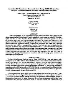
In Table 10 we report state-level predictions for the percentage of CRP land that would have converted to crops if all parcels had been forced to exit the program in 1997. Standard errors for the predictions were estimated by bootstrap. We re-sampled an equal number of NRI point-clusters from our main sample (with replacement) and obtained a new set of estimates and predictions. We repeated this exercise 1,000 times. The confidence intervals are constructed using the 0.025 and 0.975 quantiles from the 1,000 ordered predictions in each state. The spatial distribution of predictions is also illustrated in Figure 1, which displays a U.S. map with countylevel predictions.
Points on the map (randomly scattered within counties) represent acres
remaining in CRP in 1997; the shadings of the counties represent the average estimated likelihood acres will return to crop production upon exit from CRP. In areas where there are few points, the standard errors are large. Both the table and the map show wide geographic variation in the predicted likelihood that parcels will return to crop production upon exit from CRP. Together with the summary of predictions, these results imply that removal of land from crop production is at least partially irreversible throughout much of the U.S. 29
Conclusion This study examines land use choices on parcels formerly enrolled in the Conservation Reserve Program, the nation’s largest environmental program targeting land use. Even if the program continues indefinitely, it is unlikely to enroll the same parcels over time. By examining a unique set land parcels that exited the program, we gain insight into the CRP’s longer-term impacts. We find that over 38% of the land that exited CRP after 1995 (either by choice or by having their re29
The predictions of post-CRP land use are calibrated using parcels that opted out of CRP approximately one year prior to observing their subsequent use. It is possible some farmers intended to convert their land back to crops but had not yet done so. In certain areas, however, a large proportion of former CRP land did return to crops in this timeframe. This suggests enough time had elapsed for farmers to transition to their intended land use.
23
enrollment bids rejected) did not return to crop production in 1997. We predict that 42% of the acres that remained (or newly enrolled) in CRP in 1997 would not have returned to crop production if they had been forced to exit. Of the land that did not return to crop production, a majority of it remained covered with the same or similar vegetation as that which was contracted under. These estimates are robust across different econometric specifications and to Heckmanbased estimates that account for potential sample selection issues associated with the nonrepresentative sample of parcels that we use to calibrate our econometric model. We also find the predicted likelihood of a parcel returning to crop production varies widely depending on several key observable factors, including the profitability of cropping activities, the land cover contracted under CRP, other land attributes, and location. Our estimates of cropland re-establishment upon CRP contract expiration are in the range of the lowest found previous research based on stated preferences or linear programming models. 30 Because a substantial share of land did not return to crop production despite the increase in crop net returns since 1986, the results suggest a degree of rigidity in land use. 31 The fact that not all land returns to crop production could also reflect the fact that some of the land that entered CRP might have exited crop production even in the absence of the program. Nevertheless, another simulation study based on NRI data indicates that only about 10% of lands under CRP contract would have exited crop production by 1997 in the absence of the CRP (Lubowski, Plantinga, and Stavins 2003). Given our estimate that 42% of enrolled acres would not have returned to crops in 1997 if the program had expired, this suggests that the majority of 30
Our estimates are in the lower range of previous studies, after adjusting for temporal differences in the analyses. Different periods involve different land-use rents and different lands enrolled in CRP. Using prices and CRP lands as of 1992, our model predicts 51% of CRP land returning to crops, below the estimates of 53%, 63%, 57% for the 1990 and 1993 SWAC surveys and De La Torre Ugarte (1995), respectively. 31 Despite increases in crop rents, changes in farm policy might also have reduced incentives for some exiting CRP landowners to return to crop production after 1996. Under the 1996 Federal Agriculture Improvement and Reform (FAIR) Act, landowners could receive certain government payments based on historical planted acreage, while these payments had been previously “coupled” to actual plantings. If these payments determined the desirability of cropping for some landowners, this could help explain their choice not to return to crop production upon CRP exit.
24
this land would not have been removed crop production in the absence of CRP. This implies that the CRP has induced significant reductions in cropland that endure beyond the life of the program. This suggests that the CRP’s environmental benefits, as well any potentially negative employment or other economic impacts from CRP’s reduction of cropping activity, are likely to endure beyond the tenure of the contracts. Our analysis also suggests that other proposed programs targeting land-use change, such as tree planting subsidies to encourage carbon sequestration, might have land-use impacts that extend beyond the tenure of the policy. Future research could examine land-use choices in the 2002 NRI to develop a better understanding of the persistence of the land-use decisions estimated by our study. Rigidities in land-use change may arise due to fixed costs of land-use conversion and option values associated with the delay of land-use decisions in the presence of uncertainty (Schatzki 2003). 32
This behavior might also arise due to transactions costs or liquidity
constraints. In future work, researchers may wish to examine the relevance of these and perhaps other causes of these rigidities. In line with earlier findings, our analysis indicates the probability CRP land returns to crop production upon exit from the program depends on the land contracted under CRP. Lands covered with trees and wildlife practices are less than half as likely to return to crops as compared to lands covered with grasses and/or legumes. Most of this difference, however, appears to stem factors associated with land cover, not land cover itself. This finding suggests greater focus on tree planting and wildlife practices may modestly increase the enduring impacts of CRP. This idea is already embodied in the design of the Environmental Benefits Index (EBI) used in ranking landowner bids during CRP sign-ups, with greater points allocated under the 32
Given that CRP enrollment implies a loss of flexibility over land-use decisions for 10 to 15 years, some landowners may have exited CRP in order to gain the option to convert to a different land use at some future point. Landowners that do not convert to crops upon CRP exit may still plan to eventually do so. Some of the observed rigidities in land use may thus dissipate over time.
25
“enduring benefits” factor (N4) for enrollments including tree planting and habitat restoration. The magnitude of the enduring benefits from increasing enrollments under tree and wildlife practices, however, will depend on the factors determining the initial choice of CRP practice. Our predictions suggest that some parcels that were induced into planting tree and wildlife covers are more likely to return to crop production upon exit than parcels establishing tree and wildlife covers without inducements. The fact that cropland retirement often persists beyond the tenure of contracts implies initial enrollment of land in CRP yields a greater impact on land retirement per dollar than subsequent re-enrollments of the same acres.
In an extreme case, consider a policy that
disallows re-enrollment of CRP—new enrollments must be cropland not formerly enrolled in CRP. Our results suggest some land enrolled CRP would not return to crop production upon contract expiration. When added to newly enrolled acreage, these acres amount to a greater amount of land effectively retired for the same expense. The policy most effective at achieving long-term cropland reduction is unlikely to be so extreme and could be implemented by offering premium rental rates to landowners enrolling in CRP for the first time.
These first-time
premiums would be most cost-effective if calibrated according to the likelihood a parcel would be converted back to crops upon contract termination. Key factors that would enter such a calibration include the profitability of crop production relative to other uses, geographic location, specific land attributes, and perhaps land cover contracted under CRP.
26
References Akaike, Hirotugu. 1974. “A New Look at Statistical Model Identification.” IEEE Transactions on Automatic Control AU-19, pp. 719-722. Alig, Ralph J. and Robert G. Healy. 1987. “Urban and Built-Up Land Area Changes in the United States: An Empirical Investigation of Determinants.” Land Economics, 63(3), pp. 215-226. Alig, Ralph J., Michael R. Dicks, and Robert J. Moulton. 1998. “Land Use Dynamics Involving Forestland: Trends in the U.S. South.” In Kluender, R.A., N.B. Smith and M. M. Corrigan, Proceedings of the 1988 Southern Forest Economics Workers Meeting, pp. 923. Moticello, AR: University of Arkansas. Anselin, Luc. 1988. Spatial Econometrics: Methods and Models. Kluwer Academic Publishers: Boston, MA. Barbarika, Alex. 2001. Conservation Reserve Program: Program Summary and Enrollment Statistics as of August 2001, Farm Service Agency, U.S. Department of Agriculture, Washington, DC. Barlowe, Raleigh. 1986. Land Resource Economics. Prentice Hall: Upper Saddle River, N.J. Bell, Kathleen and Elena Irwin. 2001. “Modeling the Rural-Urban Interface: Data-Rich Environments.” Prepared for the AAEA Annual Meeting, Spatial Analysis Learning Workshop, Chicago, IL. Bockstael, Nancy E. 1996. "Modeling Economics and Ecology: The Importance of a Spatial Perspective." American Journal of Agricultural Economics, 78 (5), pp.1168-1180. Bockstael, Nancy E. and Kathleen Bell. 1997. “Land Use Patterns and Water Quality: The Effect of Differential Land Management Controls.” In Just, R. and S. Netanyahu, eds. International Water and Resource Economics Consortium: Conflict and Cooperation on Transboundary Water Resources. Kluwer Publishing, pp. 169-191. Carlson, Curtis, Dallas Burtraw, Maureen Cropper, and Karen Palmer. 2000. “Sulfur Dioxide Control by Electric Utilities: What are the Gains from Trade?” The Journal of Political Economy, 108(6), pp. 1292-1326. Claassen, Roger L. 1993. Rural Land Use in South Carolina 1982-1987: A Discrete Choice Approach. M.S. Thesis. Claassen, Roger and Abebayehu Tegene. 1999. “Agricultural Land Use Choice: A Discrete Choice Approach.” Agricultural and Resource Economics Review, 28(1), pp. 26-36.
27
Cooper, Joseph C. and C. Tim Osborn. 1998. "The Effect of Rental Rates on the Extension of Conservation Reserve Program Contracts." American Journal of Agricultural Economics, 80, pp. 184-194. De La Torre Ugarte, Daniel G., Daryll E. Ray, Richard L. White, and Michael R. Dicks. 1995. "The Conservation Reserve Program." The 1995 Farm Bill: A Special Series of Alternative Policy Analyses, No. 5. Agricultural Policy Analysis Center, University of Tennessee. Diaconis, Persi. and Shahshahani, Mehrdad. 1984. “On Non-Linear Functions of Linear Combinations.” SIAM Journal of Scientific and Statistical Computing, 5, pp. 175-191. Diebel, Penelope L., Larry L. Janssen, Kevin Smith. 1998. Economic and Environmental Implications of Expiring Conservation Reserve Program Contracts. Final NC-214 Committee Report. Feather, Peter, Daniel Hellerstein, and Leroy Hansen. 1999. “Economic Valuation of Environmental Benefits and the Targeting of the Conservation Programs: The Case of the CRP.” Agricultural Economics Report No. 778. U.S. Department of Agriculture Economic Research Service. Washington, D.C. Friedman, Jerome H. and Stuetzle, Werner. (1981) “Projection Pursuit Regression.” Journal of the American Statistical Association, 76, pp. 817-823. Hardie, Ian W. and Peter J. Parks. 1996. “Program Enrollment and Acreage Response to Reforestation Cost-Share Programs.” Land Economics 72(2), pp. 248-260. Heckman, James J. (1978). “Dummy endogenous variables in a simultaneous equation system.” Econometrica, 46, pp. 931-959. Heckman, James J. (1979). “Sample selection bias as a specification error.” Econometrica, 47, pp. 153-162. Hsieh, Wen-hua, Elena G. Irwin, and Lynn Forster. 2001. “Spatial Dependence among County Level Land Use Changes.” Manuscript. Irwin, Elena G. and Nancy E. Bockstael. 2002. “Interacting Agents, Spatial Externalities, and the Endogenous Evolution of Residential Land Use Pattern.” Journal of Economic Geography, 2(1). Irwin, Elena G., Wen-hua Hsieh, and Lawrence W. Libby. 2002. “The Effect of Rural Zoning on the Spatial Allocation of Urban Land.” Manuscript. Johnson, Philip N., Sukant K. Misra, and R. Terry Ervin. 1997. “A Qualitative Choice Analysis of Factors Influencing Post-CRP Land Use Decisions.” Journal of Agricultural and Applied Economics, 29(1), pp.163-173.
28
Lichtenberg, Erik. 1989. "Land Quality, Irrigation Development, and Cropping Patterns in the Northern High Plains." American Journal of Agricultural Economics, 71(1), pp. 187-194. Lubowski, Ruben N. 2002. Determinants of Land-Use Transitions in the United States: Econometric Analysis of Changes among the Major Land-Use Categories. Ph.D. Dissertation. Harvard University, Cambridge, MA. Lubowski, Ruben N., Andrew J. Plantinga, and Robert N. Stavins. 2003. “Determinants of LandUse Change in the United States, 1982-1997: Results from a National Level Econometric and Simulation Analysis.” Resources for the Future Discussion Paper No. 03-47. Washington, DC. Mauldin, Thomas E., Andrew J. Plantinga, and Ralph J. Alig. 1999a. “Determinants of Land Use in Maine with Projections to 2050.” Northern Journal of Applied Forestry, 16(2), pp. 8288. Mauldin, Thomas E., Andrew J. Plantinga, and Ralph Alig. 1999b. “Land Use in the Lake States Region: An Analysis of Past Trends and Projections of Future Changes.” U.S. Department of Agriculture, Forest Service. Pacific Northwest Research Station, Research Paper PNW-RP-519. Miller, Douglas J. and Andrew J. Plantinga. 1999. “Modeling Land Use Decisions with Aggregate Data.” American Journal of Agricultural Economics, 81(1), pp. 180-194. Osborn, Tim. 1997. “New CRP Criteria Enhance Environmental Gains,” Agricultural Outlook, AO-245. (http://www.ers.usda.gov/publications/agoutlook/oct1997/ao245e.pdf) Parks, Peter J. and Randall A. Kramer. 1995. "A Policy Simulation of the Wetlands Reserve Program." Journal of Environmental Economics and Management, 28, pp.223-240. Parks, Peter J. and James P. Schorr. 1997. “Sustaining Open Space Benefits in the Northeast: An Evaluation of the Conservation Reserve Program.” Journal of Environmental Economics and Management 32, pp. 85-94. Plantinga, Andrew J. 1996. "The Effects of Agricultural Policies on Land Use and Environmental Quality." American Journal of Agricultural Economics, 78(4), pp.10821091. Plantinga, Andrew J., Ralph Alig, and Hsiang-tai Cheng. 2001. “The Supply of Land for Conservation Uses: Evidence from the Conservation Reserve Program.” Resources, Conservation and Recycling, 31, pp. 199-215. Plantinga, Andrew J. and SoEun Ahn. 2002. “Efficient Policies for Environmental Protection: An Econometric Analysis of Incentives for Land Conversion and Retention.” Journal of Agricultural and Resource Economics 27(1), pp. 128-145.
29
Roberts, Michael J. and Shawn Bucholtz. "Slippage in the Conservation Reserve Program or Spurious Correlation? A Comment.” Forthcoming in the American Journal of Agricultural Economics. Schatzki, Todd. 2003. “Options, Uncertainty, and Sunk Costs: An Empirical Analysis of Land Use Change.” Journal of Environmental Economics and Management 46, pp. 86-105. Skaggs, R.K., R.E. Kirskey and W.M. Harper. 1994. "Determinants and Implications of PostCRP Land-Use Decisions." Journal of Agricultural and Resource Economics 19(2), pp. 299-312. Stavins, Robert N. and Adam B. Jaffe. 1990. "Unintended Impacts of Public Investments of Private Decisions: The Depletion of Forested Wetlands." American Economic Review, 80(3), pp. 337-352. Tiebout, C.M. 1956. "A Pure Theory of Local Expenditures." The Journal of Political Economy, 64, pp.416-424. U.S. Department of Agriculture Economic Research Service. “Agricultural Resources and Environmental Indicators.” 2003., Ralph Heimlich, ed. Agriculture Handbook No. 722. Washington, D.C. Venables, W.N. and B.D. Ripley. 1994. Modern Applied Statistics with S-Plus. Springer: New York, NY. Wood, Simon N. 2000. “Modelling and Smoothing Parameter Estimation with Multiple Quadratic Penalties.” Journal of the Royal Statistical Society Series B, 62(2), pp. 413428. Wu, Junjie. 2000. "Slippage Effects and the Conservation Reserve Program." Journal of Agricultural Economics 82, pp. 979-992.
30
American
Data Appendix Cropland Net Returns:
Estimated annual cropland net returns per acre consist of two
components: a weighted average of the net returns per acre for 21 major crops based on prices, yields, costs, and acres, and total federal farm program payments per acre, excluding conservation payments for cropland retirement.
We used state-level marketing-year-average
prices and county-level yields from the National Agricultural Statistics Service (NASS) for all crops (barley, all dry edible beans, corn, cotton, flaxseed, alfalfa hay, other hay, oats, peanuts, potatoes, rye, rice, sorghum, soybeans, sugarcane, sugar beets, sunflowers, tobacco, winter wheat, durum wheat, other spring wheat). We assume that landowners base their expectations of future land-use returns using current price levels and the average value of yields over the previous five years. In this way, we smooth over idiosyncratic weather shocks that affect yields in particular years. We use the current commodity price because time-series of most commodity prices show strong degree of autocorrelation—price shocks are far more persistent than yield shocks.
Data on cash costs as a percentage of revenue at the state and regional level,
respectively, are from the Census of Agriculture and USDA Economic Research Service’s (ERS). County acreage data from the National Agricultural Statistics Service (NASS) and the Census of Agriculture provided weights for averaging across individual crops.
County-level
estimates of total federal program payments per acre are from the Census of Agriculture and include receipts from deficiency payments, support price payments, indemnity programs, disaster payments, and payments for soil and water conservation projects. We excluded payments from the Conservation Reserve and Wetlands Reserve programs (CRP and WRP), which are reported jointly in the Census, because we examine the CRP as a distinct land-use category.
31
Pasture Net Returns: Annual net returns per acre for pasture were estimated using pasture yields from the National Cooperative Soil Survey (NCSS) averaged for each county using NRI soils and acreage data. We multiplied these yields by the state price for “other hay” from NASS and subtracted costs per acre for hay and other field crops from the Census of Agriculture.
Range Net Returns: Annual net returns per acre for rangeland were estimated using forage yields from NCSS, weighted with NRI soils and acreage data and multiplied by state-level per head grazing rates for private lands from the ERS database on cash rents.
Costs for range
management are assumed to be borne by the tenant and thus reflected in the grazing rates.
Forest Net Returns: We estimate annual forestry net returns per acre by annualizing at a 5 percent interest rate the net present value of a weighted average of sawtimber revenues from different forest types based on prices, yields, costs, and acres. State-level stumpage prices were gathered from a variety of state and federal agencies and private data reporting services. Regional merchantable timber yield estimates for different forest types were obtained from Richard Birdsey of the U.S. Forest Service. Regional replanting and annual management costs were derived from Moulton and Richards (1990) and Dubois, McNabb and Straka (1999). The net present value of an infinite stream of forestry revenues for each forest type was calculated using an optimal rotation age determined with the Faustmann formula, assuming forests start at year zero in a newly planted state. County acreage and sawtimber output data from the Forest Inventory and Analysis (FIA) and Timber Product Output (TPO) surveys of the U.S. Forest Service provided weights for averaging across individual forest types and species, respectively.
32
Urban Net Returns: Annual urban net returns per acre are estimated as the median value of a recently-developed parcel, less the value of structures, annualized at a 5 percent interest rate. This measure corresponds to the average annual rents from an acre of improved bare land and is based on value of land for the construction of single-family homes, which is the primary use of developed land at the national scale. Median county-level prices for single family homes were constructed from the decennial Census of Population and Housing Public Use Microdata Samples and the Office of Federal Housing Enterprise Oversight (OFHEO) House Price Index. Regional data on lot sizes and the value of land relative to structures for single-family homes were obtained from the Characteristics of New Housing Reports (C-25 series) and the Survey of Construction (SOC) micro data from the Census Bureau. Further details on the construction of the urban net returns are provided in Plantinga, Lubowski, and Stavins (2002).
More complete descriptions and citations of data sources are provided in Lubowski (2002) and are available from the authors upon request.
33
Appendix Supplement Projection pursuit To examine the robustness of our model to model specification we consider adapted a non-parametric projection pursuit model, which has greater flexibility than (3) and (4), to our discrete choice model. In theory, rents determine the probability that land will be converted to cropland. Our county-level proxies, however, cannot capture the great heterogeneity of land within counties. In the second model, we attempted to account for heterogeneity by interacting parcel-level characteristics with county-level rent estimates. These interactions, however, may be non-linear, and the interactions may differ across parcels in complex ways.
These
complexities could arise due to the many margins on which land use can change, irreversibilities associated with many land-use changes, and the heterogeneity of land and demography within U.S. counties. For these reasons, and because our goal is to predict land-use transitions rather than to test specific forms of land-use rent functions, we examine this more flexible statistical model to predict land-use transitions. The projection pursuit model assumes f(X) has the following semi-parametric structure: f(X)= α0 + ∑ f i (α Tj X ), J
(5)
j =1
where α0 is a constant, X an (N x K) matrix of explanatory variables, J a chosen number of onedimensional non-parametric projections, each denoted by fj(), and each αj a unit-length column vector with K elements that defines the orientations of the projections. This model allows for non-linearity and complex interactions between the explanatory variables. It has the advantage of being relatively parsimonious yet un-restrictive in terms of the functional form. For large enough J, this model can approximate arbitrary continuous functions (e.g., Diaconis and
34
Shahshahani 1984). Despite the generality of the functional form, it is feasible to estimate functions with high dimensionality (large K). Friedman and Stuetzle (1981) proposed a projection-pursuit regression method for estimation of (5) when Y is observed. Statistical software is available (such as in S-Plus and R) to estimate this model. This software does not, however, contain packages that fit projection pursuit models to discrete choice or categorical data. Although existing statistical packages do not estimate the above model with a binomial response, there are well-developed methods and statistical packages to estimate a similar model having the form: f(X) = α0 +
K
∑ f (x ) , k =1
k
k
(6)
where the response can take on any distribution from the exponential family, including the binomial logit and probit. Models with the general form in (6) belong to a family called generalized additive models (GAM). The difference between (5) and (6) is that the smooth nonparametric functions in (6) are fit along the axes of the explanatory variables rather than in carefully chosen directions—the model does not allow for interactions between the explanatory variables. We estimate our model by combining continuous-response projection pursuit regression with a binomial-response GAM. We do this in two stages. In the first stage, we naively estimate the projection pursuit model by substituting the 0-1 indicator of cropland conversion in place of the continuous variable Y. Because this model is estimated using least squares, the estimate is inefficient. From this initial regression, however, we retain set of carefully chosen projections ( αˆ j ) that we use to transform our explanatory variables into J projections. We denote each projection by zj = αˆ Tj X . We then estimate the GAM:
35
f(X) = α0 +
∑ f (z ) . J
j =1
j
j
(7)
Key model selection decisions include the number of projections (J) and the methods used for fitting the smooth functions fi(zj). We chose J by inspection of the improvement in fit. We found the fit of the model improved only modestly beyond two projections (relative to the degrees of freedom used). A second benefit of the projection pursuit model is that, when J = 2, we can visually compare the location of the data we use for estimation (the parcels that dropped out of CRP) with the out-of-sample data (those remaining in CRP in 1997). At least with respect to the data we observe, we can see how far from our sample data we must extrapolate in order to make predictions about CRP contracts as a whole. The smooth projections were estimated using penalized regression splines. Each line zj is divided into an ordered set of points known as knots. On each interval between the knots, a constrained cubic polynomial is fit to the data. The line is constrained to be continuous and have continuous first derivatives, so the line is smooth at each knot. The key decision is the number of knots to choose for each smooth function. This decision was made using an un-biased risk estimator (UBRE) that maximizes fit less a penalty for the equivalent number of parameters used by the cubic splines. 33
33
We used the R statistical packages “modreg” written by Brian Ripley and “mgcv” written by Simon Wood (2000). R is public domain statistical software available free at http://www.r-project.org/. These sources provide more detail on projection pursuit, the generalized additive model, and the UBRE model selection criterion.
36
Table 1 Summary Statistics: Means and Standard Deviations of Parcel-Level Variables 1
Variable
EXIT PLANTCRO P
SIGNUP
COVER-TW
1
Description
Equals 1 if exited CRP from 1992 to 1997, 0 otherwise. Equals 1 if land is in crops in 1997 after exiting CRP, 0 otherwise. Equals 1 if land enrolled in CRP signups 1 through 5, 0 otherwise. Equals 1 if contracted CRP cover practice is trees or wildlife habitat, 0 otherwise.
Parcels in CRP in 1992 and/or 1997 (N=21,172)
Parcels in CRP in 1992
Parcels in CRP in 1997
Parcels exiting CRP, 1992-1997
Parcels remaining in CRP, 1992-1997
Parcels exiting and in crops in 1997
Parcels exiting and not in crops in 1997
(N=19,785)
(N=18,416)
(N=2,756)
(N=17,029)
(N=1,596)
(N=1,160)
0.0986 (0.2981)
0.1051 (0.3066)
0.00 (0.00)
1.00 (0.00)
0.00 (0.00)
1.00 (0.00)
1.00 (0.00)
0.0617 (0.2406)
0.0657 (0.2478)
0.00 (0.00)
0.6256 (0.4840)
0.00 (0.00)
1.00 (0.00)
0.00 (0.00)
0.5825 (0.4931)
0.6170 (0.4861)
0.5567 (0.4968)
0.8173 (0.3864)
0.5934 (0.4912)
0.7832 (0.4122)
0.8745 (0.3314)
0.0959 (0.2944)
0.0943 (0.2923)
0.0975 (0.2967)
0.0811 (0.2730)
0.0960 (0.2944)
0.0343 (0.1813)
0.1598 (0.3666)
EI
Erodibility index.
13.10 (14.72)
13.01 (14.34)
13.12 (14.78)
12.94 (14.16)
13.02 (14.37)
12.48 (13.48)
13.70 (15.20)
PRIME
Equals 1 if designated prime farmland, 0 otherwise.
0.2873 (0.4525)
0.2848 (0.4513)
0.2839 (0.4509)
0.3182 (0.4658)
0.2809 (0.4494)
0.3429 (0.4748)
0.2770 (0.4477)
SLOPE
Slope percentage.
4.30 (4.41)
4.26 (4.33)
4.23 (4.39)
4.88 (4.47)
4.19 (4.30)
4.76 (4.14)
5.08 (4.96)
Data are weighted by the acreage weights provided by the NRI.
37
Table 2 Attrition from the Conservation Reserve Program 1992-1997 CRP Contracted Cover Practice2 Grasses and/or Legumes Trees and/or Wildlife Habitat All
CRP Status in 1997 (acres, % of acres, standard error of %) Total 3 Continue in CRP Exit CRP 27,543,700 3,287,000 30,830,700 89.3 % 10.7 % 100 % (0.1) (0.1) 2,921,200 290,200 3,211,400 91.0 % 9.0 % 100 % (0.4) (0.4) 30,464,900 3,577,200 34,042,100 89.5 % 10.5 % 100 % (0.1) (0.1)
1
Estimates are from the National Resources Inventory (NRI) on the 19,785 survey points that were reported in the CRP in 1992. Percentages in each cell are of total acres in the specified contracted cover practice. Standard errors are based on the NRI’s stratified sampling design. 2 These are general categories reported by the NRI that include the more specific practices contracted for under the CRP.
38
Table 3 1997 Use of Lands that Exited CRP CRP Contracted Cover Practice2 Grasses and/or Legumes Trees and/or Wildlife Habitat All
Crops 2,161,800 65.8 % (0.5) 76,100 26.2 % (2.5) 2,237,900 62.6 % (0.6)
Land Use in 1997 1 (acres, % of acres, standard error of %) Pasture Forest Urban Range Other3 771,700 23.5 % (0.4) 37,800 13.0% (1.7) 809,500 22.6 % (0.4)
22,700 0.7 % (0.1) 161,700 55.72 % (2.2) 184,400 5.15 % (0.3)
1
5,000 0.1 % (0.0) 2,300 0.8 % (0.5) 7,300 0.5 % (0.2)
288,400 8.8 % (0.3) 8,800 3.0 % (0.8) 297,200 8.3 % (0.3)
37,400 1.1 % (0.1) 3,500 1.2 % (0.4) 40,900 1.1 % (0.1)
Total 328,700 100 % 290,200 100 % 3,577,200 100 %
Estimates are from the National Resources Inventory (NRI) based on 2,756 survey points that exited CRP between 1992 and 1997. Standard errors are based on the NRI’s stratified cluster sampling design. 2 These are general categories in the NRI that subsume the more specific practices contracted for under the CRP. 3 Includes rural roads, water bodies, barren lands, and “other” farm and non-farm lands, as designated by the NRI.
39
Table 4 Summary Statistics: Means and Standard Deviations of County-Level Variables 1
Variable
Description
Parcels in Parcels in Parcels in CRP in CRP in CRP in 1992 1992 1997 and/or 1997 (N=21,172) (N=19,785) (N=18,416) 81.98 80.74 80.50 (51.75) (50.84) (51.19)
Parcels exiting CRP, 1992-1997
Parcels remaining in CRP, 1992-1997
Parcels exiting and in crops in 1997
Parcels exiting and not in crops in 1997
(N=2,756) 95.59 (54.81)
(N=17,029) 79.00 (50.07)
(N=1,596) 105.05 (54.24)
(N=1,160) 79.77 (52.06)
CROPS
Crop net returns ($/acre/year) 1
Δ CROPS
Change in crop net returns from 1986 2
71.71 (60.61)
70.59 (59.40)
70.04 (58.29)
87.01 (77.09)
68.67 (56.66)
95.01 (86.76)
73.64 (54.91)
GOV PAYMENTS
Government payments ($/acre/year)
8.89 (5.01)
8.86 (5.01)
8.85 (5.01)
9.25 (4.92)
8.81 (5.02)
9.67 (4.34)
8.56 (5.70)
Δ GOV PAYMENTS
Change in government payments from 1986
-17.75 (10.39)
-17.63 (10.36)
-17.39 (10.27)
-21.05 (10.97)
-17.23 (10.21)
-22.92 (10.20)
-17.92 (11.48)
PASTURE
Pasture net returns ($/acre/year)
27.51 (22.17)
27.05 (22.03)
27.19 (22.11)
30.48 (22.40)
26.65 (21.95)
29.86 (18.74)
31.52 (27.43)
Δ PASTUR
Change in pasture net returns from 1986 base
32.30 (28.86)
31.66 (28.69)
31.93 (28.85)
35.70 (28.79)
31.18 (28.64)
33.60 (24.29)
39.22 (34.77)
FOREST
Forest net returns ($/acre/year)
12.27 (15.42)
12.19 (15.39)
12.26 (15.38)
12.42 (15.75)
12.16 (15.34)
10.25 (13.16)
16.06 (18.78)
Δ FOREST
Change in forest net returns from 1986
6.79 (10.60)
6.69 (10.47)
6.75 (10.54)
7.15 (11.09)
6.64 (10.39)
5.99 (9.22)
9.08 (13.43)
RANGE
Urban net returns ($/acre/year)
11.06 (11.79)
11.22 (11.85)
11.26 (11.65)
9.19 (12.87)
11.46 (11.71)
8.02 (13.60)
11.16 (11.28)
Δ RANGE
Change in urban net returns from 1986
-0.13 (3.13)
-0.01 (3.15)
-0.15 (3.12)
-0.09 (3.23)
-0.12 (3.14)
0.51 (3.19)
-0.61 (3.18)
URBAN
Range net returns ($/acre/year)
2,437 (1,826)
2,427 (1,756)
2,435 (1,826)
2,453 (1,843)
2,424 (1,746)
2,401 (1,458)
2,540 (2,349)
Δ URBAN
Change in range net returns from 1986
-166 (434)
-172 (427)
-176 (430)
-76 (456)
-183 (423)
-4 (386)
-197 (532)
E
1 2
Data are weighted by the acreage weights provided by the NRI. Values are in real 2001 dollars, adjusted by the producer price index for all commodities. The net return change variables are the difference between 1996 and 1986 real values.
40
Table 5 Model Selection Statistics for Alternative Specifications Rho
Model
Specification
Spatial Surface Yes
Simple linear No Linear with interactions (AIC minimum) Linear with all twoway interactions
Yes No Yes No
1
Joint Model 0.42 (0.13) 0.54 (0.13) 0.36 (0.14) 0.51 (0.13) 0.47 (0.14) 0.60 (0.12)
% Deviance Explained Selecti on Model 8.6% 7.7% 9.4% 8.0% 10.7% 10.1%
1
Main Mode l 24.1 % 17.0 % 25.6 % 19.6 % 27.9 % 22.7 %
2
Joint Model 10.6% 9.6% 12.5% 10.8% 14.0% 12.6%
Akaike Information Criterion (AIC) 3 Selectio Main Joint n Model Model Model 2,784. 2,321.4 461.9 4 2,827. 2,335.4 492.1 9 2,722. 2,281.7 438.6 3 2,748. 2,291.1 455.3 4 2,828. 2,343.1 483.4 5 2,849. 2,347.0 500.8 8
Rho is the estimated error term correlation between the selection and the main equations. Standard errors for rho are in parentheses. 2 Calculated relative to a model with only a constant in the equation(s) of interest. 3 AIC was computed using one observation per sample cluster. AIC= -2*(log likelihood)+2*(number of parameters).
41
Table 6 Linear Model with Interactions (AIC Minimum) and Spatial Surface Selection Model Second Stage Dep. Var.=EXIT Dep. Var.=PLANTCROPS Estimate Std. Error Estimate Std. Error INTERCEPT -0.930 0.532* 0.900 0.728 SIGNUP 0.065*** 0.726 COVER-TW 0.342 0.202* 0.106 0.353 EI -0.003 0.003 0.001 0.007 PRIME 0.040 0.072 0.157*** 0.609 SLOPE 0.003 0.007 -0.063 0.034* CROPS 0.000 0.001 0.001*** 0.005 GOV PAYMENTS 0.009 0.006 0.012** 0.03 PASTURE 0.004*** 0.002 0.007 -0.012 RANGE 0.000 0.004 0.003 0.002 FOREST 0.005*** -0.011 0.012 -0.015 URBAN 0.000 0.000 0.000 0.000 Δ CROPS 0.001 0.001* 0.001** 0.002 Δ GOV PAYMENTS 0.004*** 0.014 0.009 -0.014 Δ PASTURE 0.003*** -0.009 0.005* 0.011 Δ RANGE -0.013 0.017 Δ FOREST 0.011 0.006* 0.012 0.017 Δ URBAN 0.000 0.000 0.000 0.000 SIGNUP*FOREST 0.006 0.003* SIGNUP*RANGE -0.003 0.003 SIGNUP*Δ RANGE 0.022 0.012* COVER-TW*CROPS -0.004 0.002* COVER-TW*GOV PAYMENTS -0.023 0.016 COVER-TW*PASTURE 0.007** 0.018 COVER-TW*RANGE -0.002 0.012 COVER-TW*FOREST 0.006*** -0.004 0.016 0.022 COVER-TW*URBAN 0.000 0.000 COVER-TW*Δ GOV PAYMENTS 0.007*** 0.021 COVER-TW*Δ PASTURE 0.004*** -0.018 EI*CROPS 0.000*** 0.000 EI*PASTURE 0.000*** 0.001 EI*RANGE 0.000 0.000 EI*URBAN 0.000 0.000 EI*Δ CROPS 0.000 0.000 EI*Δ PASTURE 0.000 0.000 0.000 0.000 EI*Δ URBAN 0.000*** 0.000 PRIME*GOV PAYMENTS -0.025 0.015* PRIME*URBAN 0.000 0.000 0.000 0.000 PRIME*Δ CROPS 0.000 0.001 PRIME*Δ FOREST -0.011 0.007 SLOPE*PASTURE -0.002 0.001 SLOPE*FOREST 0.001 0.001 SLOPE*URBAN 0.000 0.000 0.000 0.000 SLOPE*Δ GOV PAYMENTS -0.002 0.001 SLOPE*Δ PASTURE 0.002 0.001* SLOPE*Δ FOREST -0.003 0.002 SLOPE*Δ URBAN 0.000 0.000 HECKMAN ODDS RATIO 0.384 (0.1626**) Observations N=21,162 Log Likelihood -8,805.468 1 Spatial surface coefficients not reported. *Significant at 10%; ** Significant at 5%; *** Significant at 1%. Explanatory Variables 1
42
Table 7 Predictions for Acreage Returning to Crop Production Predicted % of Acres Returning to Crop Production in 1997 Model
Specification
Actual (see Table 2)
Spatial Surfac e
In Sample (Exited CRP) Grass Trees or All or Wildlife Parcels Legume Cover Cover
Out of Sample (In CRP in 1997) Grass Trees or All or Wildlife Parcels Legume Cover Cover
n/a
63
66
26
n/a
n/a
n/a
Yes
61
64
24
58
61
30
No
60
63
24
58
62
29
Yes 1
61 (52-69)
64 (56-72)
24 (14-39)
58 (51-65)
61 (55-67)
31 (19-48)
No
61
64
26
59
62
31
Yes
61
64
25
59
62
32
No
61
64
26
59
62
34
Simple linear
Linear with interactions (AIC minimum) Linear with all twoway interactions 1
95% confidence interval for predicted percentage reported in parentheses. Estimates in bold indicate selected model.
43
Table 8 Sensitivity of Predictions to Changes in Net Returns Variables Predicted % of Acres Returning to Crop Production in 1997 1
Scenario
Variable
Change in 1996 Level 2
Original results (See Table 7)
In Sample (Exited CRP) Grass Trees or All or Wildlife Parcels Legume Cover Cover
Out of Sample (In CRP in 1997) Grass Trees or All or Wildlife Parcels Legume Cover Cover
61
64
24
58
61
30
Crop net returns (CROPS)
+50
69
73
31
66
69
37
-50
51
54
19
50
52
23
Government payments (GOV PAYMENTS) Pasture net returns (PASTURE)
+50
67
70
30
64
67
36
-50
55
58
20
52
55
25
+50
58
61
22
55
58
28
-50
64
67
27
61
64
32
Forest net returns (FOREST)
+50
62
65
25
59
62
30
-50
61
65
24
58
61
30
Range net returns (RANGE)
+50
62
65
25
60
63
31
-50
60
63
24
57
60
29
Urban net returns (URBAN)
+50
55
58
22
52
54
26
-50
67
70
27
64
68
34
1
Predictions are estimates from linear model with interactions (AIC minimum) and spatial surface (see Table 6). Predictions based on the indicated percentage change in the 1996 levels of a particular variable (e.g. CROPS) as well as on the corresponding new values for the 1986 to 1996 change in this variable (e.g. Δ CROPS).
2
44
Table 9 Sensitivity of Predictions to Cover Type for Counties with Parcels under Both Cover Types Predicted % of Acres Returning to Crop Production in 1997 Scenario
Original cover types 2 Original cover types reversed 3 All parcels put under trees/wildlife All parcels put under grass/legumes
In Sample (Exited CRP) Grass or Trees or All Legume Wildlife Parcels Cover Cover
1
Out of Sample (In CRP in 1997) Grass or Trees or All Legume Wildlife Parcels Cover Cover
58
65
32
57
63
39
51
41
54
52
48
54
50
--
50
50
--
50
60
60
--
59
59
--
1
Predictions are estimates from linear model with interactions (AIC minimum) and spatial surface (see Table 6). Predictions based on subset of 5,615 NRI parcels in 340 counties containing CRP lands in both grass/legume and trees/wildlife covers. This subset includes 1,362 parcels under grass/legume and 4,253 under trees wildlife. 3 All parcels under grass/legumes cover hypothetically assigned to trees/wildlife and vice versa. Reported predictions correspond to parcels under each of the new cover types after this hypothetical switch. 2
45
Table 10 Predicted Share of CRP Acres Returning to Crops 1 State
Land in CRP Acres (000)
Land Returning Immediately to Crops if CRP Expires Acres (000) Percent (with 95% confidence interval) 48-State Total 33,891.70 19,752.8 58 (52 - 65) North Dakota 3,331.80 2,540.30 76 (67 - 89) Montana 3,407.40 2,386.70 70 (63 - 80) Texas 4,031.00 1,596.60 40 (29 - 46) Kansas 2,656.00 1,538.10 58 (50 - 65) Iowa 1,857.60 1,500.00 81 (76 - 85) Minnesota 1,695.30 1,440.60 85 (78 - 90) South Dakota 1,431.10 1,126.20 79 (70 - 86) Colorado 2,203.10 1,049.80 48 (38 - 58) Missouri 1,542.50 987.5 64 (55 - 70) Nebraska 1,135.90 835.8 74 (67 - 78) Illinois 963.2 729.5 76 (58 - 81) Washington 1,276.60 556.3 44 (37 - 51) Wisconsin 634.2 527.2 83 (75 -89) Idaho 789.4 418.6 53 (31 - 61) New Mexico 593 278.1 47 (29 - 63) Michigan 306.1 272.7 89 (78 - 94) Indiana 294 241.4 82 (75 - 87) Ohio 295.2 236.8 80 (71 - 88) Oklahoma 1,023.90 227.6 22 (16 - 29) Kentucky 312.5 208.3 67 (59 - 75) Oregon 455.5 208.1 46 (27 - 66) Wyoming 277.8 190.1 68 (58 - 81) Mississippi 871.4 169.7 19 (13 - 29) Tennessee 246.1 103.6 42 (36 - 53) Pennsylvania 118.9 99.1 83 (60 - 96) Arkansas 164.8 67.2 41 (26 - 57) Alabama 482.6 63.4 13 (6 - 27) Utah 201.1 58.3 29 (17 - 40) Louisiana 203.9 55.9 27 (16 - 48) New York 59.3 48.4 82 (51 - 95) North Carolina 113.3 38.8 34 (21 - 63) Maryland 66.8 37.5 56(30 - 85) Virginia 56.2 32.7 58 (39 - 84) South Carolina 217.7 22 10 (5 - 21) Georgia 308.6 18.4 6 (2 - 11) Maine 24.1 8.3 34 (9 - 91) California 144.4 8 9 (0 - 27) Florida 86.7 4 5 (1 - 13) Delaware 6.9 2.1 30 (1 - 82) New Jersey 2.3 1.6 72 (17 - 99) West Virginia 1.6 0.9 53 (9- 100) Nevada 0.2 0 19 (2 - 61) Vermont 1.1 Connecticut 0.3 New Hampshire 0.2 Massachusetts 0.1 Arizona 0 District of Columbia 0 Rhode Island 0 1 CRP acreage is from FSA Contracts file as of November, 2002. Predictions are from linear model with interactions (AIC minimum) and spatial surface. Dashes indicate no predictions due to insufficient data or zero CRP land.
46
Figure 1 Location of CRP Contracts and Predictions for Return to Crop Production
47