c 2005 Institute for Scientific ° Computing and Information
INTERNATIONAL JOURNAL OF NUMERICAL ANALYSIS AND MODELING Volume 2, Supp , Pages 58–67
A PSEUDO FUNCTION APPROACH IN RESERVOIR SIMULATION ZHANGXIN CHEN, GUANREN HUAN, AND BAOYAN LI Abstract. In this paper we develop a pseudo function approach to obtain relative permeabilities for the numerical simulation of three-dimensional petroleum reservoirs. This approach follows the idea of an experimental approach and combines an analytical solution technique for two-phase flow with a numerical simulation technique for cross-sectional models of these three-dimensional reservoirs. The advantages of this pseudo function approach are that the heterogeneity of these reservoirs in the vertical direction and various forces such as capillary and gravitational forces can be taken into account in the derivation of the relative permeabilities. Moreover, this approach considers more physical and fluid factors and is more robust and accurate than the experimental approach. To reservoir engineers, the study of pseudo functions for the crosssectional models of different types itself is the study of numerical simulation sensitivity of displacement processes in reservoirs. From this study they can understand the reservoir production mechanism and development indices. Key Words. Reservoir simulation, pseudo function, mechanics of porous medium flow, cross-sectional model, non-dimensional cumulative production, relative permeability.
1. Introduction The derivation of relative permeabilities in laboratory experiments [3] is carried out on core samples of porous media. The displacement mechanism in such samples is restricted to homogeneous cores. Moreover, in general, gravitational forces are ignored, and the magnitude of capillary forces is assumed to be very small. The relative permeabilities derived under such restricted conditions take into account only the microscopic heterogeneity of the porous media and viscous forces. If they were applied to the numerical simulation of a three-dimensional reservoir model, computational indices would be better than those observed in real situations. For a three-dimensional reservoir, the depth of each layer in the vertical direction is typically of the order of 10 m, and the permeability difference between different layers is of 10 times more. The heterogeneity in permeability can lead to the viscosity increase in a water-displacing-oil or gas-displacing-oil process; consequently, water or gas is produced at the very early stage from oil wells, and the amount of water or gas dramatically increases in these wells. Also, for such a reservoir, the density difference between the displacing fluid and displaced fluid often leads water and gas to the bottom and top of oil layers, respectively. Even for a homogeneous reservoir, the interface between different fluids can be non-homogeneous. In reality, capillary forces exist. The gravitational and capillary forces have very different influences on Received by the editors September 23, 2004. 2000 Mathematics Subject Classification. 35K60, 35K65, 76S05, 76T05. 58
A PSEUDO FUNCTION APPROACH IN RESERVOIR SIMULATION
59
water and oil layers. The water layers can easily lead to the equilibrium of fluid motion in the vertical direction, and the layers with a lower water saturation can suck water from the layers with a higher water saturation under the influence of the capillary forces. But for the oil layers, the capillary forces offset the gravitational forces in those layers with a lower permeability, and this effect leads water in the higher permeability layers to the lower permeability layers. These two forces influence each other. This paper studys how to incorporate these complex forces (viscous, gravitational, and capillary) into the derivation of relative permeabilities for a three-dimensional reservoir. By reducing this reservoir to a two-dimensional cross-sectional reservoir and taking into account these forces in this reduced model, the relative permeabilities are obtained using the idea of the classical experimental approach and applied to the numerical simulation of the original three-dimensional reservoir. The computational development indices for this reservoir can accurately reflect various displacement mechanism factors in the study of numerical simulation sensitivity. The difference between our pseudo function approach and other earlier approaches [4, 5, 6] lies in the fact that we combine pseudo functions with the sensitivity study by reservoir engineers and we derive these functions by combining analytical solution and numerical reservoir simulation techniques. The physical concepts in our approach is clear, its derivation is mathematically rigorous, and it is applicable to different reservoirs. The rest of this paper is outlined as follows. In the next section we review the analytical solution technique. Then, in the third section we describe the derivation of relative permeabilities. In the fourth section we apply our pseudo function approach to a reservoir example. Finally, concluding remarks are given in the final section. 2. Analytical Solution of Two-Phase Flow For a two-phase (e.g., water and oil) flow problem in a porous medium, Buckley and Leverett obtained an analytical solution in 1942 [1]. To combine the present pseudo function approach with an analytical solution approach, in this section we briefly review the derivation of this analytical solution. 2.1. Two-phase flow. For the flow of two incompressible, immiscible fluids in a porous medium, the mass balance equation for each of the fluid phases in the x-direction is ∂sw ∂uw (2.1) φ + = 0, ∂t ∂x ∂so ∂uo + = 0, ∂t ∂x where w denotes the water phase, o indicates the oil phase, φ is the porosity of the medium, and sα and uα are, respectively, the saturation and volumetric velocity of the α-phase, α = w, o. The volumetric velocities uw and uo are given by the Darcy law Krw (sw ) ∂p , (2.3) uw = −K µw ∂x (2.2)
(2.4)
φ
uo = −K
Kro (so ) ∂p , µo ∂x
60
Z. CHEN, G. HUAN, AND B. LI
where K is the absolute permeability of the porous medium, p is the pressure, and µα and Krα are the viscosity and relative permeability of the α-phase, respectively, α = w, o. In addition to (2.1)–(2.4), the customary property for the saturations is (2.5)
sw + so = 1.
The unknowns for the system of equations (2.1)–(2.5) are sα , uα , and p, α = w, o. 2.2. Characteristics. We introduce the phase mobility functions λα (sα ) =
Krα (sα ) , µα
α = w, o,
and the total mobility λ(sw ) = λw (sw ) + λo (1 − sw ). The fractional flow functions are defined by fw (sw ) =
λw (sw ) , λ(sw )
fo (sw ) =
λo (1 − sw ) . λ(sw )
We also define the total velocity (2.6)
u = uw + uo .
By (2.1), (2.2), and (2.5), we see that ∂u = 0, ∂x
(2.7)
so u is constant in x. Because uw = fw (sw )u, it follows that (2.8)
∂uw ∂u dfw (sw ) ∂sw ∂sw = fw +u = uFw (sw ) , ∂x ∂x dsw ∂x ∂x
where the distribution function of saturation is Fw (sw ) =
dfw (sw ) . dsw
Now, we substitute (2.8) into (2.1) to see that (2.9)
φ
∂sw ∂sw + uFw (sw ) = 0. ∂t ∂x
This equation defines a characteristic x(t) along the interstitial velocity v by (2.10)
dx uFw (sw ) = v(x, t) ≡ . dt φ
Along this characteristic, it follows from (2.9) that sw is constant. Namely, it holds that (2.11)
∂sw dx ∂sw dsw (x(t), t) = + = 0. dt ∂x dt ∂t
A PSEUDO FUNCTION APPROACH IN RESERVOIR SIMULATION
61
2.3. Non-dimensional cumulative production. We consider a tube Q in the x-direction with cross-sectional area A, and we define the cumulative liquid production along this tube Z t (2.12) U (t) = A u dt. 0
From (2.10), along the characteristic x(t) we see that Z t Z Fw (sw ) t dx = u dt, φ 0 0 so, by (2.12), (2.13)
x(sw , t) =
Fw (sw ) U (t). φA
The non-dimensional fluid cumulative production is defined by ¯ (t) = U (t) , U φAL
(2.14)
where L is the length of Q. Let swe be the value of saturation at x = L. Then it follows from (2.13) and (2.14) that ¯ (t) = U
(2.15)
1 . Fw (swe )
Also, we introduce the water cumulative production Z t Z t (2.16) Uw (t) = fw dU (t) = A uw dt, tB
tB
where tB is the water break-through time (i.e., the saturation equals the critical value swc at t = tB ) and we used (2.12) and the fact that uw = fw (sw )u. Define the non-dimensional water cumulative production ¯w = Uw . U φAL
(2.17)
It follows from (2.16) and integration by parts that µ ¶ Z t Z t 1 1 ¯ Uw = fw dU (t) = fw U − U dfw , φAL tB φAL tB so, by the fact that dfw = Fw dsw , we see that µ ¶ Z t ¯w = 1 U Fw dsw . U fw U − φAL tB Then we apply (2.15) to obtain (2.18)
¯w = fw (swe ) − (swe − swc ). U Fw (swe )
Similarly, we define the oil cumulative production Z t Z (2.19) Uo (t) = fo dU (t) = A tB
tB
and the corresponding non-dimensional one (2.20)
t
¯o = Uo . U φAL
uo dt,
62
Z. CHEN, G. HUAN, AND B. LI
It is easy to see that ¯o = 1 − fw (swe ) + (swe − swc ), U Fw (swe )
(2.21) and
¯ =U ¯w + U ¯o . U
(2.22)
3. Derivation of Relative Permeabilities In an experimental approach, water and oil relative permeabilities are derived as follows: After the water and oil cumulative productions and the pressure drop are obtained, the relative permeabilities are found in an inverse fashion from the derivation of the analytical solution in the previous section. This idea also applies to the present pseudo function approach. In the approach in this paper, we think of the computational results from a cross-section model of a three-dimensional reservoir as the experimental results, and then the derivation of relative permeabilities is carried out in the same manner. 3.1. The derivation of formulas. We define the mobile resistance ratio λo (swc ) , (3.1) r(sw ) = λ(sw ) and we scale the space dimension by x . L Then we define the non-dimensional resistance ratio Z 1 (3.2) R= r(sw ) d¯ x. x ¯=
0
Note that, by (2.13) and (2.15), ¯ dFw , d¯ x=U so (3.2) becomes Z (3.3)
Fw (swe )
R=
1 Fw (swe )
¯ dFw = rU
Fw (swc )
that is, (3.4)
Z
Z
Fw (swe )
r dFw ; Fw (swc )
Fw (swe )
RFw (swe ) =
r dFw . Fw (swc )
Set Fwe = Fw (swe ). From (3.4), we see that d(RFwe ) . dFwe We also introduce the non-dimensional quantity ¯o + swc U (3.6) γ= . ¯ U (3.5)
r=
Substituting (2.15) and (2.12) into (3.6) gives (3.7)
γ = 1 − fw + sw Fwe .
We differentiate γ with respect to Fwe to have dγ dfw dsw =− + sw + Fwe , dFwe dFwe dFwe
A PSEUDO FUNCTION APPROACH IN RESERVOIR SIMULATION
63
so that, by the definition of Fw , dγ = sw . dFwe
(3.8) It follows from (3.7) that (3.9)
fw = 1 − γ + sw Fwe .
Now, by the definition of fw and (3.1), we calculate Krw and Kro as follows: (3.10)
Krw (sw ) =
µw fw (sw ) Kro (swc ), µo r(sw )
(3.11)
Kro (sw ) =
1 − fw (sw ) Kro (swc ). r(sw )
3.2. Steps for calculating Krw and Kro . We now summarize the steps for calculating Krw and Kro . For a cross-sectional model, the computation of production is performed under a fixed pressure condition. Below Q(t) denotes the instantaneous production at time t, and ∆p indicates the pressure drop at the two ends of a cross-section. Now, the steps for calculating Krw and Kro are as follows: • Record Uw , Uo , Q, and ∆p at time t; • Calculate the non-dimensional cumulative production ¯w = Uw , U ¯o = Uo , U ¯ =U ¯w + U ¯o ; U φAL φAL • Compute the non-dimensional mobile resistance ratio ∆p Qi (3.12) R= , ∆pi Q where ∆pi and Qi are the initial pressure drop and production, respectively; • Evaluate Fwe and γ by ¯o + swc U 1 ; Fwe = ¯ , γ = ¯ U U • Find the relationship between r, sw and Fwe by d(RFwe ) dγ , sw = ; dFwe dFwe • Obtain the relationship between fw and Fwe according to the equation r=
f (sw ) = sw Fwe + 1 − γ; • Calculate Krw and Kro by Krw (sw ) =
µw fw (sw ) Kro (swc ), µo r(sw )
Kro (sw ) =
1 − fw (sw ) Kro (swc ). r(sw )
4. An Application In the final section we study the pseudo function approach and verify its correctness by simulating a numerical example of waterflooding. For the computation of each cross-sectional model, we need to record the following quantities: • the triple (φ, A, L), • the initial production and pressure drop and the corresponding ones at any time after the water break-through time, and • the water and oil cumulative productions.
64
Z. CHEN, G. HUAN, AND B. LI
We then calculate the water and oil relative permeabilities using the approach outlined in §3.2. We compare our pseudo function approach with an experimental approach for a three-dimensional model which is heterogeneous in the vertical direction and homogeneous in the horizontal direction. The experimental approach is applied directly to this model to obtain the relative permeabilities. To apply the pseudo function approach, we weight-average the absolute vertical permeability of the three-dimensional reservoir with the depth of each layer as the weight to obtain a cross-sectional two-dimensional model. Then the pseudo function approach is applied to this reduced two-dimensional model and is compared with the experimental approach for the original three-dimensional model. layer K × 10−3 µm2 swc (frac) pcmax (MPa) pcmin (MPa) 1 10 0.21 0.3730 -0.4636 2 20 0.22 0.2637 -0.3278 3 40 0.23 0.1865 -0.2318 4 70 0.24 0.1409 -0.1752 5 100 0.25 0.1179 -0.1466 6 200 0.26 0.0834 -0.1036 7 400 0.27 0.0589 -0.0733 8 700 0.28 0.0444 -0.0554 9 1,000 0.29 0.0373 -0.0463 10 2,000 0.30 0.0263 -0.0327 Table 1. The distribution of vertical permeabilities. sw 0.280 0.305 0.3266 0.3483 0.3699 0.3915 0.4131 0.5 0.6 0.7 0.8 1.0
Krw 0.0 0.001 0.003 0.006 0.01 0.015 0.021 0.035 0.048 0.065 0.085 0.2
Kro 1 0.809 0.707 0.606 0.513 0.421 0.369 0.26 0.15 0.07 0.0 0.0
pc (MPa) 4.4580132E-02 6.9950912E-03 4.2926008E-03 2.4362588E-03 1.0780764E-03 2.3129978E-05 -8.3082396E-04 -3.2011603E-03 -5.0774538E-03 -6.8351193E-03 -9.1273598E-03 -5.5419870E-02
Table 2. The relative permeability and capillary pressure data. ps (MPa) gas solubility µo (mPa.s) oil volume factor (frac) oil compressibility (1/MPa)
11.2 29.5 15.5 1.0795 0.00045
9 23.2 19.7 1.0632 0.00045
6 14.3 26.3 1.0415 0.00045
3 6.98 37.6 1.0208 0.00045
0.6 1.2 52.8 1.0057 0.00045
Table 3. The oil PVT data. We now consider a concrete example where there are 10 layers with the permeability in the top layer equal to 10 × 10−3 µm2 and in the bottom layer equal to 2, 000 × 10−3 µm2 . Thus this example is highly heterogeneous in the vertical
A PSEUDO FUNCTION APPROACH IN RESERVOIR SIMULATION
65
direction, and the permeability difference between the top and bottom layers is 200 times more. The permeabilities in other layers are stated in Table 1 where pcmax and pcmin denote the maximum and minimum values of the capillary pressure (i.e., at swc and 1), respectively. Other physical and fluid data are given in Tables 2–4 where ps means the saturated pressure. item unit Data N X, N Y, N Z 20, 1, 10 Dx m 25 DY m 250 DZ m 1 perforated zone depth m 1,100 temperature C 74 initial pressure MPa 11.2 ps MPa 3 φ frac 0.3 final time year 20 water density g/cm3 1.015 water volume factor 1.022 µw mPa.s 0.42 water compressibility 1/MPa 0.00045 oil density g/cm3 0.972 µo mPa.s 37.6 oil compressibility 1/MPa 0.0003 gas weight 0.5615 oil-water viscosity ratio 89.5 injection-production pressure drop MPa 8 Table 4. The data for the three-dimensional model. The relative permeabilities obtained by the experimental approach are shown in Fig. 1 and these functions obtained by the pseudo function approach are displayed in Fig. 2. The comparison between the oil cumulative productions using these two approaches is illustrated in Fig. 3, which shows that the productions are almost identical. 5. Concluding Remarks In this paper we have developed a pseudo function approach to derive relative permeabilities for the numerical simulation of three-dimensional reservoirs. This approach combines an analytical solution technique for a two-phase flow problem and a numerical simulation technique for cross-sectional models of three-dimensional reservoirs. It follows the idea of the laboratory experimental approach and takes into account various complex factors in porous medium flow. The study of this approach can be combined with the study of numerical simulation sensitivity by reservoir engineers. Furthermore, the physical concepts in this approach is clear, its derivation is mathematically rigorous, and it is applicable to different reservoirs. References [1] S. E. Buckley and M. C. Leverett, Mechanism of fluid displacement in sands, Trans. Am. Inst. Min. Metall. Eng. 146 (1942), 107–116. [2] Z. Chen, G. Huan, and B. Li, An improved IMPES method for two-phase flow in porous media, Transport in Porous Media 54 (2004), 361–376.
66
Z. CHEN, G. HUAN, AND B. LI
Krw & Kro
0.80
0.60
0.40
0.20
0.00 0.00
0.20
0.40
0.60
0.80
Sw
Relative Permeabilities Krw & Kro
Fig. 1: The experimental relative permeabilities.
Krw & Kro
0.80
0.60
0.40
0.20
0.00 0.00
0.20
0.40
0.60
0.80
Sw
Pseudo Relative Permeabilities Krw & Kro
Fig. 2: The pseudo relative permeabilities.
[3] K. H. Coats, R. L. Nielsom, M. H. Terhune, and A. G. Weber, Simulation of threedimensional, two-phase flow in oil and gas reservoirs, Soc. Per. Eng. J. 12 (1967), 377–388. [4] C. L. Hearn, Simulation of stratified waterflooding by pseudo relative permeability curves, J. Pet. Tech. 7 (1971), 805–813. [5] J. R. Kyte and D. W. Berry, New pseudo functions of control numerical dispersion, Soc. Pet. Eng. J. 8 (1975), 269–274. [6] H. H. Jacks, O. J. E. Smith, and C. C. Mattax, The modeling of a three-dimensional reservoir with a two-dimensional reservoir simulator-The use of dynamic pseudo functions, Soc. Pet. Eng. J. 6 (1973), 175–185.
A PSEUDO FUNCTION APPROACH IN RESERVOIR SIMULATION
67
60.0
50.0
Vo (%)
40.0
30.0
20.0
10.0
0.0 0.0
4.0
8.0 12.0 Time (year)
16.0
Recovery vs T for 2-D & 3D Models
Fig. 3: The comparison of oil productions: •=experimental, –=pseudo. Department of Mathematics, Box 750156, Southern Methodist University, Dallas, TX 752750156, USA E-mail:
[email protected] URL: http://faculty.smu.edu/zchen Department of Mathematics, Box 750156, Southern Methodist University, Dallas, TX 752750156, USA E-mail:
[email protected] and
[email protected]