A Simulation – Optimization Approach in ...

E-proceedings of the 36th IAHR World Congress 28 June – 3 July, 2015, The Hague, the Netherlands

A Simulation – Optimization Approach in Development of Operation Policy for a Multipurpose Reservoir (1)

(2)

PRIYANK J. SHARMA , P. L. PATEL (1)

& V. JOTHIPRAKASH

(3)

Research Scholar, Sardar Vallabhbhai National Institute of Technology Surat, Surat - 395007, India, [email protected] (2)

Professor, Sardar Vallabhbhai National Institute of Technology Surat, Surat - 395007, India, [email protected] (3)

Professor, Indian Institute of Technology Bombay, Mumbai - 400076, India, [email protected]

ABSTRACT In the present study, behaviour of a reservoir system, Ukai reservoir, India has been examined by using a simulation model with reservoir sedimentation and flood control operating scenarios. A standard operating policy (SOP) based simulation model has been developed considering historical reservoir data of 36 years from 1975 – 2010. The system behaviour has been assessed using statistical performance indices like reliability, resilience and vulnerability. The simulation results indicated that the system is highly reliable for water supplies on one hand, and vulnerable to flood damages on the other. Keeping in view the need to optimize the system with the objective of minimizing the flood damages, ensuring reliable water supply for municipal and industrial, and irrigation demands, a monthly time stepped backward recursive stochastic dynamic programming (SDP) model has been developed while giving due consideration to target releases and target storage for monsoon periods with appropriate flood control constraints. In the SDP model, initial reservoir storage and inflow, in a particular month, have been treated as state variables; and stochasticity of inflows are addressed by computing one-time-step transition probabilities. The reservoir storage and inflow each have been discretized into seven class intervals. The optimal reservoir releases and optimal end of the period storages are reported for different combinations of state variables. The optimal policies are synthesized and rule curves are proposed for the optimal operation of Ukai reservoir. The simulation-optimization approach indicates an improvement in the reservoir operation in terms of increasing storage volumes, ensuring reliable releases, and decrease in spill events compared to existing operating conditions. Keywords: Standard operating policy, Statistical performance indices, Stochastic dynamic programming, Simulationoptimization, Ukai reservoir 1.

INTRODUCTION

The operation of a multipurpose reservoir is a challenging problem for the water resources planners and managers, for meeting spatial and temporal demand of water in command area. The southwest monsoon is the major source of water supplies for replenishment of the reservoirs in India. The divergent uses of the reservoir, i.e. for conservation, flood mitigation and power generation, give rise to conflicts in decision making. The irrigation demand need water conservation by filling up the reservoir at the end of the monsoon, while the flood control warrants empty space for absorbing high inflows, thereby creating conflicts in space and time. Further, the hydropower generation requires certain head of water to be maintained in the reservoir, which creates conflicts in discharge for meeting the consumptive use demands in the command area. In the past decade, many advances were made in the field of water resources with the adoption of different optimization techniques for planning and management of complex water resources systems. The two approaches widely adopted for planning and operation of reservoir systems are simulation and optimization. The choice of approach in analyzing the problem depends upon the availability of the data, nature or type of the objective function and its binding constraints, and the system configuration. The optimization techniques exhibit high efficiency when coupled with simulation modelling and offers better results in reservoir management problems (Fayaed et al., 2013). Simulation is a process of mimicking the dynamic behaviour of systems over the time (Karamouz et al., 2003). The simulation models adopted in reservoir operation and management are generally based on reservoir continuity or mass balance equation, and represent the hydrological behaviour of the systems considering inflows and other operating conditions (Rani and Moreira, 2010). Majority of simulation models for reservoir operations are devised to simulate a sequence of discrete time periods. The time step of the simulation model depends upon the system characteristics being simulated and nature of problem being addressed. Sigvaldson (1976) analyzed the reservoirs of the Trent River system in Canada through a mathematical simulation model for assessing the impact of alternative operating policies on the operation of the reservoir system to deal with the water conflicts in the system. Karamouz et al. (1992) investigated the reservoir operating rules for a system of multiple reservoirs using optimization, simulation and regression analyses. The reservoir operation was initially optimized for given set of streamflows, and the set of operating rules were derived. Later, the operating rules were evaluated by a simulation model using different data sets. Simonovic (1992) proposed a methodology to bridge the gap between the research studies and their field applications by an illustrative simulationoptimization model using systems approach. Wurbs (1993) presented a detailed survey of many site-specific simulation and optimization models applied to reservoir systems that may assist in decision support systems. Harboe and Ratnayake (1993) applied simulation-optimization (SO) approach for deriving the standard operating rules for Victoria Reservoir in Mahaweli River system, Sri Lanka using a stochastic dynamic programming (SDP) model with the objective of energy 1

E-proceedings of the 36th IAHR World Congress, 28 June – 3 July, 2015, The Hague, the Netherlands

maximization. Neelakantan and Pundarikanthan (2000) proposed a backpropagation neural network model, trained to approximate the simulation model for the solution of water supply problem in Chennai city. Jothiprakash et al. (2012) developed a simulation model considering historical inflow data, and inflow data generated through artificial neural network (ANN) to assess the performance of storage policies of Vaigai reservoir system in Tamil Nadu, India. The simulation model was developed incorporating monthly and daily time steps with a planning horizon of one year. Timbadiya et al. (2013) carried out a simulation study to assess the adequacy of the revised operating rules of Ukai reservoir for flood control purpose using HEC-ResSim model. Arunkumar and Jothiprakash (2014) evaluated the performance of a multireservoir hydropower system considering different operating scenarios by estimating different statistical performance indices such as reliability, resilience and vulnerability. The simulation model addresses ‘what if’ questions, while the optimization addresses ‘what should be’ type questions. Unlike simulation models, the solutions of optimization models are based on objective functions of known decision variables that are to be maximized or minimized (Loucks et al., 2005). The optimization techniques applied by researchers to reservoir operation problems involve conventional methods like linear programming (LP), non-linear programming (NLP), dynamic programming (DP) (Yeh, 1985) and data driven or artificial intelligence approaches such as artificial neural networks (ANN), genetic algorithms (GA), Fuzzy Logic (Fayaed et al., 2013). Butcher (1971) applied SDP methodology for determining the optimal operating policies of a multipurpose reservoir, wherein the policy was stated in terms of the state of the reservoir indicated by the storage volume, and the river flow in the preceding month. Doran (1975) suggested a method for improving the computational efficiency and the accuracy of the solutions by discretizing the state variables into small number of finite sets. Klemes (1977) demonstrated that coarser discretization of reservoir storage, to avoid ‘curse of dimensionality’ problem, shall not only hamper the accuracy but also postulate unrealistic results as far as storage probability distribution is concerned. Buras (1985) formulated a SDP model while minimizing the sum of squared deviations of actual releases and final storage volumes from their respective targets and derived the schedule of seasonal optimal releases along with their probabilities of occurrence under steady-state conditions. The ‘trapping’ effect in SDP can be reduced by reducing the size of storage interval by increasing the number of storage states (Goulter and Tai, 1985). Karamouz and Vasiliadis (1992) investigated the adaptability of alternate state variable discretization schemes, and their application to the reservoir operation problems. The uncertainty in the nature of inflows was addressed by computing the inflow transition probabilities and incorporating the same in deriving steady state operation policies (Chandramouli and Umamahesh, 2003; Vedula and Mujumdar, 2004; Jothiprakash and Shanthi, 2009). Akbari et al. (2011) integrated fuzzystate SDP and multi-criteria decision making (MCDM) methods for deriving operating rules for a single objective reservoir operation problem. In the past, many studies have focused either on simulation or optimization of reservoir operation, however, only few studies addressed the combined simulation-optimization procedure in development of operation policy. Moreover, effect of a state variable discretization on the value of objective function and thereby, deriving operating rules has been less explored by the previous researchers. The present study aims to develop an operation policy of a multipurpose Ukai reservoir across River Tapi, Gujarat, India with following objectives into consideration: (i) Analyzing the behaviour of the system through a simulation model based on standard operating policy (SOP) while incorporating the storage constraints and sedimentation effects in the reservoir also; (ii) Assessing the performance of the system using various statistical performance indices such as failure index, reliability, resilience and vulnerability; (iii) Development of a SDP model considering initial reservoir storage and inflows as state variables, while final storage and releases as decision variables; (iv) Comparison of simulated and optimized model results with actual operation of the past decade. 2.

STUDY AREA

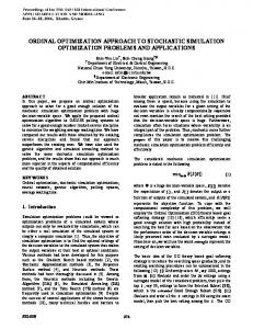
The Tapi basin is situated in the northern part of the Deccan Plateau. It extends over an area of 65,145 sq. km. The basin lies between east longitudes of 72º 38' to 78º 17' and north latitudes of 20º 5' to 22º 3'. It is bounded on the north by the Satpura range, on the east by the Mahadeo hills, on the south by the Ajanta range and the Satmala hills, and on the west by the Arabian Sea. The entire Tapi basin can be divided in three sub-basins (see Fig. 1): Upper Tapi Basin up to Hathnur, confluence of Purna with the main Tapi (29,430 sq. km.), Middle Tapi basin from Hathnur up to the Gidhade gauging site (25,320 sq. km.), and Lower Tapi basin from the Gidhade gauging site up to the Arabian sea in the Gulf of Khambhat (10,395 sq. km.). The Ukai reservoir project is a multi-purpose project, completed in 1972 initially provides benefits such as irrigation, hydropower generation, water supply to industries and drinking water for municipality, and partial flood control during the monsoon. The catchment area upto the dam site is 62,225 sq. km. The Kakrapar weir, which is 28 km downstream of Ukai dam, was constructed before 1954, supplies water in the command area through Kakrapar left bank main canal and Kakrapar right bank main canal. The different reservoir storage zones with their levels in Ukai reservoir are shown in Fig. 2. 3.

MODEL DEVELOPMENT

3.1 Standard Operating Policy (SOP) Simulation Model

Simulation is a mathematical technique which approximates the behaviour of the system for a given set of operating conditions. In present study, a SOP based simulation model has been developed for the UkaiKakrapar system. According to SOP, if the total water available (storage, St + inflow, It) at a particular period is less than the demand Dt, then all the available water is released. If the available water is more than the demand, however, less than demand + maximum storage capacity (Dt + Smax), then release is equal to the demand. On the other hand, if the available storage after meeting the demands exceeds the maximum storage capacity ((St + It) – Dt > Smax), excess water is released as spill from the reservoir. The step-wise methodology of the developed simulation model is presented as flowchart in Fig. 3. The simulation model is developed while considering different scenarios, viz. constrained scenario and sedimentation scenario, which are discussed in 2

E-proceedings of the 36th IAHR World Congress 28 June – 3 July, 2015, The Hague, the Netherlands

succeeding paragraphs. Sharma et al. (2014) presented a comparison of four different operating scenarios viz. unconstrained scenario, unconstrained scenario – I and II based on flood control guidelines given by Central Water Commission (CWC), India and a special scenario considering sedimentation effects over the long time period through a simulation model for evaluating the performance of the reservoir.

Ukai Dam

Fig. 1 Layout map of Tapi Basin (Source: iomenvis.nic.in)

Top of Dam – RL 111.25 m

Tapi River Freeboard

M.W.L. – RL 106.99 m F.R.L. – RL 105.15 m

Surcharge Storage Zone Flood Control Storage Zone

Spillway

Spillway Crest – RL 91.14 m

Conservation Storage Zone D.S.L. – RL 82.29 m

Notations:    

Ukai Dam

Under sluices

Dead Storage Zone

M.W.L. – Maximum Water Level F.R.L. – Full Reservoir Level D.S.L. – Dead Storage Level R.L. – Reduced Level

Fig. 2 Different storage zones of Ukai dam

3.1.1 Constrained Scenario In this scenario, the maximum storages in the reservoir during the monsoon are governed from flood control considerations as suggested by CWC (2000) and CWC (2008) tribunals on the basis of flood experiences of years 1998 and 2006 respectively. In the former case, the reservoir shall be filled during July and August months only, and by the end of August, the reservoir is supposed to be 95% full. While in the latter case, the reservoir shall be partly filled in July month and partly in the latter half of the September month. In the rest period, the reservoir is not filled considerably, and its levels are kept low to provide cushion for absorbing high floods. In the second case, the reservoir is supposed to be around 77% 3

E-proceedings of the 36th IAHR World Congress, 28 June – 3 July, 2015, The Hague, the Netherlands

filled by the end of August, thereby providing additional empty space to absorb high floods. In both the cases, the reservoir is required to be completely filled by October 01, for augmenting the supplies in the lean period and meeting the demands in the command area. The permissible flood control storage levels as suggested by CWC tribunals in 2000 and 2008, are presented in Table 1. For non-monsoon months, there are no constraints on the permissible storage capacity of the reservoir.

4

E-proceedings of the 36th IAHR World Congress 28 June – 3 July, 2015, The Hague, the Netherlands

Input parameters: Historical monthly inflows ( ), initial reservoir storage ( ), command area demands ( and ), evaporation losses ( )

Operating Scenario Parameters: Reservoir storage capacity ( ), Maximum , permissible flood control storage minimum reservoir storage

Calculate the Available Storage 1 = + − −

No

Check for Municipal & Industrial demand

1 ≥ Yes

=

1

=

2 = No

1 −

Check for Irrigation demand

2 ≥ Yes

=

2

=

3 =

2 −

No

+

Check for Overflows/ Spills ( )

3 ≥ Yes =

=0

=

3 −

=

3

Final Storage,

= final period of simulation

No

= +1

+1

= Yes

Estimate performance indices - Failure index, Reliability, Resilience and Vulnerability Fig. 3 Flowchart of SOP based simulation model

5

E-proceedings of the 36th IAHR World Congress, 28 June – 3 July, 2015, The Hague, the Netherlands

Table 1. Permissible flood control storage levels for Ukai reservoir as per CWC guidelines (Sharma et al., 2014) CWC guidelines - 2000

CWC guidelines - 2008

Month & Date

Reservoir storage level (metres)

Reservoir storage volume (MCM)

Reservoir storage level (metres)

Reservoir storage volume (MCM)

July 01

97.84

3825.41

97.84

3825.41

August 01

101.50

5420.67

101.50

5420.67

September 01

104.54

7058.18

102.10

5714.86

September 15

-

-

103.63

6524.02

October 01

105.15

7414.29

105.15

7414.29

3.1.2 Sedimentation Scenario In this scenario, the effect of reservoir sedimentation, which led to the modifications in the reservoir storage-elevation curve over the years, are considered in the development of SOP model. Initially, hydrographic survey of the reservoir was done in 1972, at the time of construction of dam, and the storage-elevation curve were prepared accordingly. Later, hydrographic surveys were carried out at regular intervals, and the final survey was undertaken in 2003. While analyzing the reservoir sedimentation pattern, it is seen that, at present, the live storage capacity of the reservoir is less than 9% of its original capacity. The details of change in reservoir capacity are presented in Table 2. Table 2. Effect of sedimentation on storage capacity of Ukai reservoir (Sharma et al., 2014) Reservoir storage level (metres)

1972

1979

1983

1994

2003

Dead Storage Level (DSL)

82.29

1418.5

1388.0

1160.0

882.0

684.39

Full Reservoir Level (FRL)

105.15

8511.0

8240.0

7963.0

7497.1

7414.29

Maximum Water Level (MWL)

106.99

9801.78*

9411.74

9095.35

8562.99

8480.18

Description

Reservoir storage capacity in different years (MCM)

* The storage-elevation capacity curve data for 1972 was available only till FRL i.e. 105.15 m. For higher elevation (MWL), it is extrapolated till 106.99 m, by fitting a third-order polynomial equation.

3.2 Performance Evaluation of Simulation Model The performance of the simulation model is evaluated using three statistical performance indices, viz. reliability with respect to water supply, irrigation and flood control, resilience and vulnerability with respect to flood damages. The reliability computations are made by slightly altering the concept proposed by Hashimoto et al. (1982) to incorporate a failure index, which incorporates both frequency and severity of failure (Raje and Mujumdar, 2010). The water supply and irrigation reliabilities are defined based on the deficits, i.e. unable to fulfill the demands. The failure measure is defined with respect to water supply and irrigation: = =

∆

[1] [2]

where, FMws and FMirr are the water supply and irrigation failure indices respectively, t and t are the water supply and irrigation deficits in period t respectively, DMIt and DIt are the municipal and industrial, and irrigation demands in period t respectively. Similarly, the failure measure for flood control is defined as: =

[3] − where, FMfc is the flood control failure index, t is the excess live storage over maximum storage as per flood control guidelines in period t, Kt is the reservoir capacity, and Smaxt is the maximum storage permissible as per flood control rules for the period t. The failure index (FI) is expressed as the summation of all failure measures over all the periods to the total number of simulation periods (T) in months. It is expressed as: ∑ ( ) = [4] The corresponding reliability () is then defined as  = 1 – FI. The resilience is defined as how quickly a system is likely to recover or bounce back from failure, once failure has occurred. As per Hashimoto et al. (1982), the resilience is probability of a year of success following a year of failure. Resilience () is defined with respect to flood control, where a success year denotes no spilling over, while a failure year accounts for damage due to spilling. [ ∈ , = ∈ ] [5] where, Xt is the state of output of system at time t, S is the set of all satisfactory (success) outputs, and F is the set of all unsatisfactory (failure) outputs. The vulnerability () is defined as the measure of likely damage of a failure event defined by Hashimoto et al. (1982) and the mean vulnerability was simplified by Kjeldsen and Rosbjerg (2004) as: 6

E-proceedings of the 36th IAHR World Congress 28 June – 3 July, 2015, The Hague, the Netherlands



=

1

[6]

where, vj is the excess volume over the maximum live storage (for flood control purpose)/ deficit volume than the particular demand (for irrigation and water supply purpose) of the jth failure event, M is the number of failure events. The maximum vulnerability is estimated as:  = max [7] The SOP model works on the hierarchical order, i.e., first fulfilling municipal and industrial water supply demands, then meeting irrigation demands, and after meeting all the demands if the available storage is in excess of storage capacity, overflows or spills are recorded. This has been used for the computation of vulnerability. 3.3 Stochastic Dynamic Programming (SDP) Optimization Model In present study, a backward moving monthly time-step stochastic dynamic programming (SDP) model is developed for deriving optimal operating rules for Ukai reservoir. The initial reservoir storage volume and the inflows were considered as state variables, while the final storage volume and releases from the reservoir were treated as decision variables. 3.3.1 Inflow Discretization In many SDP formulations, inflow is treated as a stochastic state variable and the stochasticity is addressed by computing inflow transition probabilities using first order Markov process (Vedula and Mujumdar, 2005). In present study, the inflow is discretized into 7 classes ranging from CI = 3 to CI = 9 using a discretization scheme proposed by Karamouz and Vasiliadis (1992). In this approach, the intervals are unequally spaced such that number of data, N(i), for each class interval are same by adjusting the width of the class interval. If N(i) is the number of data points in the ith class interval and n(i, j) is the number of data points of jth sub-interval of ith class interval (where n(i, j) < N(i)), ( , ) is the average of the lower and upper bound of the jth sub-interval; and S(i) is the number of sub-intervals in the ith class, then the characteristic value for each class interval, ( ) is computed as: ()

( )=

(, ) . ()

(, )

∀ ∈ [1, … . ,

],

( , ) ∈ [1, … . , ( )],

[8] ( ) ∈ [1, … . . ]

3.3.2 Reservoir Storage Discretization In present study, the reservoir storage volumes are discretized into equal and unequal interval storage class intervals (SI) ranging from 5 to 11, using classical scheme proposed by Karamouz and Vasiliadis (1992). Considering equal interval storage discretization, the entire active storage capacity is divided into several classes of equal class width. The characteristic storage ( ( )) is calculated as: 2 −1 ∆ , ∀ ∈ [1, … . . , ] [9] 2 where, S = storage increment, k = storage state, SI = number of storage class intervals. ( )=

In another approach, the reservoir storage is divided into different classes based on equal number of data points in each interval, thereby resulting in unequal width of storage intervals as discussed in Section 3.3.1. Here, the storage states are not further divided into sub-intervals, and the representative value for a particular class is just taken the mean of upper and lower bounds of that interval (Sharma, 2014). Thus, for different months there will be different representative storage values for corresponding storage states. Representative storage or characteristic storage state ( ( )) is calculated as: ( + ) ( )= [10] 2 where, LB and UB are lower and upper bounds values of the chosen storage state at time t. 3.3.3 Inflow Transition Probabilities The uncertainties in inflow in the SDP model are addressed by computing transition probabilities for different months. The transition probabilities are used to measure the dependence of inflow in current period t + 1 on the inflow in the preceding period t. The transition probability is defined as the probability that inflow during the period t + 1 will be in class interval j, given that inflow during the period t lies in the class interval i. Mathematically, = [ = / = ] [11] where, It = i , in Eq. (11), indicates that inflow during period t belongs to discrete class interval i, and It+1 = j, indicates that inflow during period t+1 belongs to discrete class interval j. The assumption made in the SDP models is that streamflow series is a stationary stochastic process, which implies that transition probability matrix does not change from year to year (Mujumdar and Saxena, 2004). Therefore, for each discretization of the inflows, there shall be 12 transition matrices. 3.3.4 Storage Probability Distribution The storage probability is computed as the number of values in a particular storage state divided by the total values in different storage states in given time period. Coarse discretization of state variables resulted in skewed probability distribution, and finer the distribution (i.e. by increasing the number of storage states), ‘trapping’ phenomenon can be avoided (Goulter and Tai, 1985). 3.3.5 Objective Function 7

E-proceedings of the 36th IAHR World Congress, 28 June – 3 July, 2015, The Hague, the Netherlands

The objective function used in present study is the same as adopted by Loucks et al. (1981, 2005), Buras (1985), and Jothiprakash and Shanthi (2004). The SDP model minimizes the annual sum of squared deviations of actual releases from desired target releases and actual storage volume from desired target storage volumes. The computations start from a distant period in future, and recursing the optimal values backward till steady state is reached. [(

=

−

) +(

−

) ]

[12]

where, k = initial storage state at beginning of time period t, i = inflow state in time period t, l = final storage state at the end of time period t, t = time period (here, months), Bkilt = system performance, Rt = release from the reservoir during time period t, TRt = target release during time period t, St = initial storage at the beginning of time period t, and TSt = target storage to be maintained at the beginning of time period t. 3.3.6 Constraints The objective function (Eq. 12) is subjected to the following model constraints: (a) Reservoir continuity equation The mass balance in the reservoir from one time step to another time step is given by storage continuity equation as: = + − − − , ∀ = 1, 2, … … , 12 [13] where, St+1 = final storage during the month t, It = inflow during the month t, Et = evaporation losses in the reservoir during time t, and Ot = overflows or surplus from the reservoir during time t. (b) Release constraints The release from the reservoir in a particular month should be less than or equal to estimated or target releases. The release constraint is expressed as: 0≤ ≤ , ∀ = 1, 2, … … , 12 [14] (c) Reservoir storage constraints The reservoir storage during a given month should neither be more than its maximum permissible storage capacity, nor less than its minimum storage capacity. This constraint is mathematically described as: ≤ ≤ , ∀ = 1, 2, … … , 12 [15] where, Smin = minimum storage capacity of the reservoir in million cubic metres (Mm 3), and Smax = maximum permissible storage capacity of the reservoir in Mm3. (d) Reservoir evaporation loss constraints Reservoir evaporation losses during time period, t is function of reservoir storage at that point of time. The desired expression for evaporation losses can be expressed as: )/2], = + [( + ∀ = 1, 2, … … , 12 [16] Here, at and bt = regression coefficients. (e) Over flow constraints The overflow constraint takes care of the spills as and when the storage in the reservoir exceeds the maximum capacity of the reservoir. The relevant constraint can be expressed as: = − , ∀ = 1, 2, … … , 12 [17] [18] and ≥ 0, ∀ = 1, 2, … … , 12 4.

RESULTS AND DISCUSSION

4.1 SOP Simulation Model vis-à-vis Actual Operation The methodology (see Fig. 4) for the simulation model of the system has been programmed in MATLAB®, and the runs were taken for a period of 36 years, i.e. 420 monthly time steps from June 1975 to May 2010. The simulation model incorporated two different scenarios, i.e. constrained scenario and sedimentation scenario representing the actual condition of the reservoir system. The performance of the simulation model has been assessed by estimating various statistical performance indices, viz. reliability, resilience and vulnerability. From the results, water supply reliability for fulfilling municipal and industrial demands was found to be 100% for both the cases. The results of other parameters compared with actual operation are tabulated in Table 3. Table 3. Comparison of statistical performance indices of simulation model and actual operation Mean Mean Maximum Maximum Statistical Reliability – Resilience – Reliability Resilience Vulnerability – Vulnerability – Vulnerability – Vulnerability – Performance Flood Flood – Irrigation – Irrigation Irrigation Flood control Irrigation Flood control indices control control 6 3 6 3 6 3 6 3 (10 m ) (10 m ) (10 m ) (10 m ) SOP Simulation model

0.998

0.678

1.00

0.924

21.40

1942.50

21.4

12,191

Actual operation

0.995

0.887

0.995

0.943

135.02

1742.83

135.02

11,918

8

E-proceedings of the 36th IAHR World Congress 28 June – 3 July, 2015, The Hague, the Netherlands

From Table – 3, it is seen that SOP model shows higher reliability and resilience for flood control vis-à-vis the estimated values of the said parameters for actual operating conditions. On the other hand, the reliability and resilience of the system with reference to irrigation are similar for both SOP and actual operating conditions. The higher reliability and resiliency of the system against the floods, while operating as per SOP, may be due to operation of the system on scientific and predefined guidelines. The existing system in the past was operated based on experience, and a lot of human interventions were involved for releasing the water for irrigation. 4.2 Equal Interval vis-à-vis Unequal Interval Reservoir Storage Discretization A SDP model was developed in MATLAB® wherein the inflow and initial storage volume were discretized into 7 states, considering both equal and unequal intervals for reservoir storage. In unequal interval discretization, the intervals widths are not uniform but are based upon the number of data points. This method results in better transition matrices as the nonzero entries are eliminated and each data point receives equal weightage in construction of matrix. The comparison between two discretization techniques for 5 storage states (SI = 5) for January month is shown in Fig. 4. The storage probability distribution for equal and unequal interval discretization for January month is shown in Fig. 5. It is clearly seen that unequal interval distribution yields equal storage probability distribution, while equal interval distribution portrays skewed distribution. Storage state ‘1’ refers to reservoir nearing full condition and storage state ‘5’ refers to reservoir nearing empty condition.

January (SI=5) 8000

STORAGE VOLUME (106 M3)

7000

1345.98

1934.29

6000 5000 4000 3000

1345.98

315 585

1345.98

1080

1345.98 2815.61

2000 1000 0

1345.98 684.39

684.39

Equal discretization

Unequal discretization

DSL

SI=1

SI=2

SI=3

SI=4

SI=5

Fig. 4 Equal interval discretization vis-à-vis unequal interval storage discretization for January month (SI = 5) (The values in the boxes indicate the width of class interval).

(a)

(b)

Fig. 5 Storage probability distribution for (a) equal interval discretization and (b) unequal interval storage discretization for January month (SI = 5)

9

E-proceedings of the 36th IAHR World Congress, 28 June – 3 July, 2015, The Hague, the Netherlands

The optimal values of the objective functions resulting from different combinations of inflow and initial storage states (both for equal and unequal discretization) for the month of October is shown in Fig. 6. The graphs shows the value of objective function against combination of different storage and inflow states. 9.00E+05

VALUE OF OBJECTIVE FUNCTION (MCM^2)

8.00E+05 7.00E+05 6.00E+05 CI=3 CI=4

5.00E+05

CI=5 4.00E+05

CI=6 CI=7

3.00E+05

CI=8 CI=9

2.00E+05 1.00E+05 0.00E+00 5

6

7

8

9

10

11

STORAGE STATES (a) 9.00E+05

VALUE OF OBJECTIVE FUNCTION (MCM^2)

8.00E+05 7.00E+05 6.00E+05

CI=3 CI=4

5.00E+05

CI=5 4.00E+05

CI=6 CI=7

3.00E+05

CI=8 CI=9

2.00E+05 1.00E+05 0.00E+00 5

6

7

8

9

10

11

STORAGE STATES (b) Fig. 6 Objective function values for different storage states for (a) equal interval storage discretization, and (b) unequal interval storage discretization for October month

From Fig. 6, it is evident that with the increase in storage and inflow states, the value of objective function improves, i.e. decreases, which implies that finer the discretization, better would be the value of objective function. Coarse discretization results in skewed probability distributions, and, hence by increasing the number of storage and inflow states, distributes 10

E-proceedings of the 36th IAHR World Congress 28 June – 3 July, 2015, The Hague, the Netherlands

the skewness of the distribution among other classes and a relatively less skewed distribution is obtained. Further, unequal interval discretization exhibits nearly uniform probability distribution. Hence, compared to equal interval discretization, unequal interval discretization yields better value of the objective function. Additionally, it is observed that for higher states, i.e. SI = 10 or 11, and CI = 8 or 9, that there is significant improvement in the value of the objective function under such condition. Similar trend in results were observed for other months also, however, could not be presented due to paucity of space. 4.3 Operation Policy and Rule Curves The optimal end of the month storage levels were derived and optimal operating policy was formulated based on the best combination of inflow and storage states. From the analyses, it has been found that storage state SI = 10 and inflow state CI = 8, provides the best combination for yielding the minimum value of the objective function. The operation policy has been formulated for each month that indicate the optimal end of the month storage volumes for given initial storage state Inflow State

6

3

Initial storage volume in reservoir 6 3 (10 m )

i=1

i=2

i=3

i=4

i=5

i=6

i=7

i=8

k=1

2412.70 (93.91)

2412.70 (93.91)

2412.70 (93.91)

2412.70 (93.91)

4209.50 (98.80)

4726.50 (100.00)

5420.00 (101.49)

5714.86 (102.10)

5714.86 (102.10)

k=2

4209.50 (98.80)

4209.50 (98.80)

4726.50 (100.00)

5420.00 (101.49)

5714.86 (102.10)

5714.86 (102.10)

5714.86 (102.10)

5714.86 (102.10)

5714.86 (102.10)

k=3

4726.50 (100.00)

4726.50 (100.00)

4726.50 (100.00)

5714.86 (102.10)

5714.86 (102.10)

5714.86 (102.10)

5714.86 (102.10)

5714.86 (102.10)

5714.86 (102.10)

k=4

5420.00 (101.49)

5420.00 (101.49)

5714.86 (102.10)

5714.86 (102.10)

5714.86 (102.10)

5714.86 (102.10)

5714.86 (102.10)

5714.86 (102.10)

5714.86 (102.10)

Storage State

Optimal end of the month storage volume (10 m )

(k) and inflow state (i). The operation policy for the month of September is presented in Table 4.

11

E-proceedings of the 36th IAHR World Congress, 28 June – 3 July, 2015, The Hague, the Netherlands

k=5

5997.50 (102.63)

5714.86 (102.10)

5714.86 (102.10)

5714.86 (102.10)

5714.86 (102.10)

5714.86 (102.10)

5714.86 (102.10)

5714.86 (102.10)

5714.86 (102.10)

k=6

6431.00 (103.45)

5714.86 (102.10)

5714.86 (102.10)

5714.86 (102.10)

5714.86 (102.10)

5714.86 (102.10)

5714.86 (102.10)

5714.86 (102.10)

5714.86 (102.10)

k=7

6768.50 (104.04)

5714.86 (102.10)

5714.86 (102.10)

5714.86 (102.10)

5714.86 (102.10)

5714.86 (102.10)

5714.86 (102.10)

5714.86 (102.10)

5714.86 (102.10)

k=8

7057.50 (104.54)

5714.86 (102.10)

5714.86 (102.10)

5714.86 (102.10)

5714.86 (102.10)

5714.86 (102.10)

5714.86 (102.10)

5714.86 (102.10)

5714.86 (102.10)

k=9

7155.00 (104.71)

5714.86 (102.10)

5714.86 (102.10)

5714.86 (102.10)

5714.86 (102.10)

5714.86 (102.10)

5714.86 (102.10)

5714.86 (102.10)

5714.86 (102.10)

k = 10

7307.15 (104.97)

5714.86 (102.10)

5714.86 (102.10)

5714.86 (102.10)

5714.86 (102.10)

5714.86 (102.10)

5714.86 (102.10)

5714.86 (102.10)

5714.86 (102.10)

Table 4. Operation policy from SDP model for September month # Figures in the brackets indicate reservoir levels in metres

Depending upon the initial storage level and inflow into the reservoir for a particular month, upper and lower limits of storages were obtained for the same month from the SDP model, see Fig. 7. Same procedure was adopted for other months also to obtain upper and lower bounds of storage curves for the whole year. Such curves may be the guiding principle for operating the reservoir during flood and drought conditions. 4.4 SDP Operating Policy vis-à-vis Actual Reservoir Operation The optimal operating policy obtained from the SDP model is compared with the actual reservoir operation in the last decade, i.e., from water years 2000 – 2010. The SDP rule curves were compared to the actual operation of 2000-01, 2003-04, 2006-07 and 2009-10, and it is found that the SDP rule curves are superior in a way allocating more conservation storage for the dry periods, and effectively confirming to flood control guidelines suggested by CWC, Govt. of India (see Fig. 8). Thus, the optimal operation policy obtained from present SDP model offers advantage over the existing operation condition of the same system.

Fig. 7 Operating rule curves for the reservoir with storage zones

12

E-proceedings of the 36th IAHR World Congress 28 June – 3 July, 2015, The Hague, the Netherlands

Fig. 8 Optimal monthly releases for the reservoir

5.

CONCLUSIONS

The following key conclusions can be drawn from the present study:i) The SOP based simulation model has been developed to mimic the actual behaviour of the system while considering the flood storage constraints and incorporating the long term changes in the reservoir capacity due to sedimentation. The system exhibits higher reliability for water supplies for municipal and irrigation requirements vis-à-vis flood control in the downstream reaches of the reservoir. ii) The SOP based simulation model gives higher reliability and resiliency of the system compared to the corresponding values of the parameters for actual past operating conditions of the system. iii) The SDP model results indicated that better value of objective function are achieved by adopting finer discretization of state variables. With increase in number of inflow and storage states, there is significant improvement in the value of the objective function. iv) Additionally, it is also found that unequal interval storage discretization performs better than equal interval storage discretization for higher states and, thus, yields better values of objective function. v) The optimal operating policy has been formulated for the best combination of state variables, i.e., SI = 10 and CI = 8, and stated in terms of final storage levels for given initial storage and inflow states. vi) The optimized SDP rule derived in the present study has been compared with actual reservoir operation of Ukai reservoir in the past decade, and it is found that the SDP policy would be much better for the system as it offers more conservation of water for lean periods while adhering to flood control restrictions in the monsoon periods. ACKNOWLEDGMENTS Authors wish to thankfully acknowledge the partial funds and necessary support received from Centre of Excellence (CoE) on “Water Resources and Flood Management”, TEQIP-II, Ministry of Human Resources Development (MHRD), Government of India for conducting the study reported in the paper. REFERENCES Akbari M., Afshar A., and Mousavi J. (2011). Stochastic multiobjective reservoir operation under imprecise objectives: Multicriteria decision-making approach. Journal of Hydroinformatics, 13(1), 110-120. Arunkumar R., and Jothiprakash V. (2014). Evaluation of a multi-reservoir hydropower system using a simulation model. ISH Journal of Hydraulic Engineering, 20(2), 177-187. Buras N. (1985). An application of mathematical programming in planning surface water storage. Water Resources Bulletin, 21(6), 1013-1020. Butcher WS. (1971). Stochastic dynamic programming for optimum reservoir operation. Water Resources Bulletin, 7, 1520. Chandramouli C., and Umamahesh NV. (2003). Application of stochastic dynamic programming model for multi-purpose reservoir operation. Journal of Applied Hydrology, 16(3), 38-45. Doran DG. (1975). An efficient transition definition for discrete state reservoir analysis: The divided interval technique. Water Resources Research, 11(6), 867-873. Fayaed SS., El-Shafie A., and Jaafar O. (2013). Reservoir-system simulation and optimization techniques. Stochastic Environmental Research and Risk Assessment, 27(7), 1751-1772. Goulter IC., and Tai FK. (1985). Practical implications in the use of stochastic dynamic programming for reservoir operation. Water Resources Bulletin, 21(1), 65-74. Harboe R., and Ratnayake U. (1993). Simulation of a reservoir with a standard operating rule. Extreme hydrological Events: Precipitation, Floods and Droughts, Proceedings of the Yokohama Symposium, July 1993. IAHS Pub. No. 213, pp. 421 – 428. 13

E-proceedings of the 36th IAHR World Congress, 28 June – 3 July, 2015, The Hague, the Netherlands

Hashimoto T., Stedinger JR., and Loucks DP. (1982). Reliability, resiliency, and vulnerability criteria for water resource system performance evaluation. Water Resources Research, 18(1), 14-20. Jothiprakash V., and Shanthi G. (2004). Stochastic dynamic programming model for optimal policies of a multi-purpose reservoir. Journal of the Indian Water Resources Society, 24(4), 32-42. Jothiprakash V., Shanthi G. (2009). Comparison of policies derived from stochastic dynamic programming and genetic algorithm models. Water Resources Management, 23(8), 1563-1580. Jothiprakash V., Nirmala J., and Arunkumar R. (2012). Performance assessment of storage policies of the Vaigai Reservoir using a simulation model. Water International, 37(3), 319-333. Karamouz M., Houck MH., and Delleur JW. (1992). Optimization and simulation of multiple reservoir systems. Journal of Water Resources Planning and Management, 118(1), 71-81. Karamouz M., and Vasiliadis HV. (1992). Bayesian stochastic optimization of reservoir operation using uncertain forecasts. Water Resources Research, 28(5), 1221-1232. Karamouz M., Szidarovszky F., and Zahraie B. (2003). Water Resources Systems Analysis. (Vol. 38) Boca Raton, FL: Lewis Publishers. Kjeldsen TR., and Rosbjerg D. (2004). Choice of reliability, resilience and vulnerability estimators for risk assessments of water resources systems. Hydrological Sciences Journal, 49(5), 755-767. Klemeš V. (1977). Value of information in reservoir optimization. Water Resources Research, 13(5), 837-850. Loucks DP., Stedinger JR., and Haith DA. (1981). Water resource systems planning and analysis. Prentice-Hall, New Jersey, USA. Loucks DP., Van Beek E., Stedinger JR., Dijkman JP., and Villars MT. (2005). Water resources systems planning and management: An introduction to methods, models and applications. Paris: UNESCO. Mujumdar PP., and Saxena P. (2004). A stochastic dynamic programming model for stream water quality management. Sadhana, 29(5), 477-497. Mujumdar PP., and Vedula S. (2004). Reservoir operation modelling for irrigation with stochastic inflow and rainfall. ISH Journal of Hydraulic Engineering, 10(2), 23-35. Neelakantan TR., and Pundarikanthan NV. (2000). Neural network-based simulation-optimization model for reservoir operation. Journal of Water Resources Planning and Management, 126(2), 57-64. Raje D., and Mujumdar PP. (2010). Reservoir performance under uncertainty in hydrologic impacts of climate change. Advances in Water Resources, 33, 312-326. Rani D., and Moreira MM. (2010). Simulation–optimization modelling: a survey and potential application in reservoir systems operation. Water Resources Management, 24(6), 1107-1138. Sharma PJ. (2014). Stochastic Dynamic programming model in development of operation policy for a multipurpose reservoir. M. Tech. Thesis, Sardar Vallabhbhai National Institute of Technology, Surat, India. Sharma PJ., Patel PL., and Jothiprakash V. (2014). Performance evaluation of a multi-purpose reservoir using simulation models for different scenarios. Proceedings of Conference HYDRO – 2014 International, MANIT Bhopal, India. Sigvaldson OT. (1976). A simulation model for operating a multipurpose multi-reservoir system. Water Resources Research, 12(2), 263-278. Simonovic SP. (1992). Reservoir systems analysis: closing gap between theory and practice. Journal of Water Resources Planning and Management, 118(3), 262-280. Timbadiya PV., Mirajkar AB., and Patel PL. (2013). Ukai Reservoir operation simulation using HEC-ResSim. Proceedings of Conference HYDRO – 2013 International, IIT – Madras, India. Vedula S., and Mujumdar PP. (2005). Water resources systems: Modelling techniques and analysis. Tata McGraw-Hill Education, New Delhi, India. Wurbs RA. (1993). Reservoir-system simulation and optimization models. Journal of Water Resources Planning and Management, 119(4), 455-472. Yeh WWG. (1985). Reservoir management and operations models: A state-of-the-art review. Water Resources Research, 21(12), 1797-1818.

14