Table 1: Order book table for Allianz AG, 06/01/2005, 10:30:08.35-. 10:30:12.81 showing prices (B = Buyers, S=Sellers), best bids and asks: # order number ...
A Quantitative-Behavioural Approach to Modelling Stock Market’s Microstructure ¨ ∗, Otto Loistl∗ , and Johannes Prix∗ Michael Hutl
1 Real Market Performance
on the stock as well as on the trading hours. This high rate of cancellations might be part of screen fighting2 The current market microstructure discussion deals which might not only comprise noise effects but be a with issues that are at the core of practical regulation1 rational tactical game of market participants. in the EU and the US addressing the real performance of capital markets, i.e. how orders are transformed into prices. The academic community is narrowing the gap between these real tasks and the abstract models investigating the behaviour of prices only. Among the issues treated now are (a) the differentiation between prices and orders. Prices are only the tip of the iceberg of the entire capital market performance: orders drive the market; prices are generated by matching orders according to exchanges rules and regulations. Asks Time 10:30:08.35 10:30:09.87 10:30:11.89 10:30:11.96 10:30:12.56 10:30:12.56 10:30:12.56
#
A
Limit (Size)
8 9
1 1
97.56 (600) 97.55 (250)
11
4
97.53 (436)
S #
11 11
Transaction Price (Size)
97.53 (36) 97.53 (400)
Bids B #
(Size) Limit (36) 97.53
A 1
# 7
(400) 97.53 (300) 97.52
1 1
10 21
7 10
Table 1:
Order book table for Allianz AG, 06/01/2005, 10:30:08.3510:30:12.81 showing prices (B = Buyers, S=Sellers), best bids and asks: # order number, (A)ction (1 = Insertion, 4 = Acceptance), order size and limit.
For instance, in Table 1 one observes three bid insertions between 10:30:08.35 and 10:30:12.56, where the best bid in this period was bid 7 at limit 97.53 due to the price-time priority rule of the Xetra system. The insertion of an ask at 10:30:12.56 led to a transaction price of 97.53 and full execution of order 7, 10 and 11. This is illustrated in Figure 1 which contains the information shown in Table 1 starting at 10:30:11.00 with best bid at 97.53 (order 7) and best ask at 97.56 (order 8). The white circle at 10:30:12.56 represents the two transactions described above (see Figure 1). Therefore, neglecting the entire order book means disregarding the fact that prices are generated by order matching, thus ignoring important information contained in the order activities (as shown in Table 1 and Figure 1). Furthermore, at Xetra a large part of the orders for DAX 30-stocks are cancelled (see [2, p. 31]). The magnitude of this cancellation rate depends
Figure 1: Order flow ”mountain” for Allianz AG (06/01/2005) consisting of cumulated volume for bids (green resp. light grey area) and asks (blue resp. dark grey area) and prices (white circles). (Note that the plotted limit scale (in Euro) is reverted).
(b) the fact that market events (prices or orders) occur asynchronously. The distribution of the waiting time between two market events has gained increasing interest (see, for instance, [4], [12] and [1]). However, not only waiting times vary, but also volatility is not constant over time. A prominent way of considering these facts is the generalized variance gamma model discussed by [3]. (c) Increased availability of detailed high-frequency market data advances the investigation of these issues on a causal level. In order to avoid measurement without theory an appropriate theoretical foundation for order book market analysis is required (see also [5, 8, p.3]). We present a structural-econometric approach which is based on order activities occurring at the markets microstructure level.
2 Simulation Results
∗ Chair
for Investment Banking and Catallactics, Vienna University of Economics and Business Administration, Austria 1 See EU Commission, Draft Commission Directive, implementing Directive 2004/39/EC (Brussels, 6.02.2006) and SEC, Regulation NMS, Release Nr 34/51808, August 29, 2005.
Our isomorphic model of the capital market’s microstructure enables the simulation of securities’ or2 The
term ’fighting-screen’ has been used by [15]
der flows. Figure 2 presents the result of a simula-
Figure 2:
Simulated order flow ’mountain’ consisting of cumulated volume for bids (green resp. light grey area) and asks (blue resp. dark grey area) and prices (white circles).
tion run3 of 80 market actions (order insertions, acceptances and deletions)4 on a single security market with 300 agents. The corresponding model is presented in section 3. The estimated values for the model parameters were obtained by the procedures described in section 4. The simulated order book was initialized with the entire observed Xetra order book data for Allianz AG with time stamp 06/01/2005 10:30:03. Asks Time 0 0 0.0916 0.0916 0.1526 ... 0.2242 0.2242
# 175
A Init
Limit (Size) 97.57 (200)
208 209 214 ... 221
4 4 4 ... 4
97.52 (200) 97.50 (300) 97.50 (200) ... 97.53 (400)
S #
208 209 214 ... 221 221
Transaction Price (Size)
97.54 (200) 97.54 (300) 97.54 (200) ... 97.54 (100) 97.53 (300)
Bids B #
181 181 181 ... 181 171
(Size) Limit (300) 97.53 (800) 97.54
A Init Init
# 171 181
...
...
...
Table 2:
Simulated Order book table for Allianz AG initialized with Xetra order book data with time stamp 06/01/2005, 10:30:03. Table shows prices (B = Buyers, S=Sellers), best bids and asks: # order number, (A)ction (1 = Insertion, 4 = Acceptance, Init=simulated order book initialized with Xetra order entries), order size and limit.
Table 2 illustrates the first 3 prices generated by the matching of the inserted asks with the best bid at 97.54 as shown in Figure 2 (first 3 white circles on the bid side). The determination of the shown simulated transaction prices (and volumes) by the limits (and volumes) of the observed initial orders 181 and 174 illustrates the predictive power of the entire order book for the price (and transaction volume) process 5 .
3 Quantitative-Behavioural Finance by Means of Doubly Stochastic Markov Process The performance of capital markets is generated by human beings’ actions governed by their wishes, needs and fears. That’s the basic message of behavioural finance. We follow this idea, applying a quantitative model to capture the market’s performance at the microlevel. Orders are placed at the trading place by individual agents, indicating their willingness to buy or to sell a given number of securities. Prices are generated whenever two market participants agree to exchange the quantity of securities for the amount of money indicated obeying the exchange’s rules and regulations. Further, agents process information entailed in the market’s observable behaviour. One group of traders - value traders for short - draw conclusions by observing the difference between prices and (fundamental) values6 . The other group of traders - information traders for short - draw conclusions primarily by relying on technical trading rules. For both groups of traders we have to implement their behavioural attitudes. Behavioural Finance has reaffirmed the influence and importance of individuals behavioural attitudes in markets and has shifted attention to the interactions between individuals at markets. McFadden developed the theory of discrete choice providing a probabilistic framework for modelling individual behavior by means of Random Utility Maximization (see [10]). We present a model which applies Random Utility Maximization to modelling individual actions at capital markets. We rely on the model presented in [7] to integrate discrete choice theory into a Markov process and thus modelling agents’ interactions at markets. This combination of quantitative and behavioral finance, i.e. quantitative-behavioral finance constitutes the ’mathematics of human interaction’ postulated by [2]. Figure 3 illustrates the different layers of our model. In more detail the following cornerstones of our approach can be identified:
1. Information and Value Traders Assuming a multi-agent model we distinguish between value and information traders7 . Value traders are assumed to place or delete orders to buy (sell) at limits being lower (greater) than the best ask (bid), i.e. value traders are not seeking immediate execution 3 The simulation is based on a C++ implementation of our at all costs but put high value on the achievable
model including an isomorphic implementation of the Xetra market model. 4 The simulated number of market actions equals the number of market actions observed in the Xetra order book of Allianz AG on 06/01/2005 between 10:30:03 and 10:30:17. 5 The question in how far the simulated order flow mountain distribution (here we present a single simulation run only) copes with reality is subject to current research (see [6]).
6 We rely on this differentiation at the core of real economic evaluations, even if this differentiations is neglected by our discipline’s currently prevailing paradigm which is, according to [9, p. 75], correctly characterized by the aphorism (in analogy to Oscar Wilde’s characterization of a cynic) ”Economists know the price of everything and the value of nothing”. 7 For the distinction between these two types of traders see [14].
ξ ,ξ
,ξ
,ξ
I.2 Functional form Value = ξ ipφikip + ξ realφikreal + ε ik U ik
Generating Procedure Estimated by discrete choice theory based Maximum Likelihood methods from order book data Obtained by adapting trading strategies and multi-factor models
U ikInfo = ξ ip 'φikip ' + ξ trd φiktrd + ε ik I.3 Value Trader: Fundamental Value piext Representing (a) Economic data and (b) Company data
Derived from financial analyst opinions (target prices and recommendations)
I.4 Information Trader: Technical trading price pitech
Estimated from order book data
II. Market Performance II.1 Order book � Entire set of bids and asks scaled in time intervals of 1/100 secs
Agents‘ decisions to place orders are determined by Random Utility Maximization
II.2 Transaction
Prices are determined by order matching based on the exchange‘s rules and regulations
Figure 3:
Doubly Stochastic Markov Process
Data For Evaluation of utility/willigness to pay or sell
Basic Data / Variables I Utility Function I.1 Behavioural parameters ip real ip ' trd
pik ) and φreal ik is the price realization potential measuring the likelihood of a trade (as function of pik and the best bid and ask limit). The i-th information trader evaluates the order acceptance at limit pik according to 0
0
trd trd Φik = ξ ip φip φik ik + ξ
(3)
0
where φip ik denotes the individual preference potential measuring the expected profit in terms of opportunity costs (as function of ptech and pik ). φtrd i ik is the volume realization potential measuring the likelihood of a trade (as ratio of the targeted volume q(pik ) and the available market volume Qk at limit pik ). By weighting these utility potentials by the behav0 ioural parameters ξ ip and ξ real (resp. ξ ip and ξ trd ) the agent tackles the tradeoff between targeting a high expected return and realizing the order on the market.
Layers of Modelling Stock Market Performance
3. Random Utility Maximization Given this specification of the discrete choice model transaction price. Each value trader i is represented and assuming the stochastic utility part ²ik to be by a scalar draw pext from a value distribution H(x) Gumbel distributed, the Logit choice probability for i obtained from financial analysts’ opinions. action aik that agent i chooses to place/accept an Information traders on the other side bet on a order at limit pik is given by change of the price due to new information obtained exp(Φik ) by technical analysis. The information trader’s P (Uik > Uil , l 6= k) = PKi (4) investigation generates information which in his or l=1 exp(Φil ) her eyes is not reflected in the traded price. As the where K is the number of action alternatives of the i value of new information diminishes as soon as it is i-th agent. Further, the deletion of an order with limit reflected in the price, information traders put high p already placed by value trader i is assumed to ik value on execution speed. In our model information take place whenever the trader’s random utility U il traders accept orders placed by value traders. Hence, for any other limit p 6= p is higher than the utility il ik while value traders determine the transaction price, U for the placed order limit p 10 . The probability of ik ik information traders determine the transaction vol- a deletion is given by 1 − P (U > U , l 6= k). ik il ume. Each information trader is modelled by a draw ptech from a technical trading price distribution G(x). 4. Doubly Stochastic Markov Process i 2. Utility Function and Behavioural Parameters The i-th agent’s k-th action alternative is to place, accept or delete8 a limit order9 at limit pik for q(pik ) units of the security. Following [7] we specify the random utility function for an action alternative k by Uik = Φik + ²ik
(1)
where Uik has the functional form of a multi-factor model (see, for instance, [11]). The representative utility is adapted from [7] as follows. For the i-th value trader the deterministic utility Φik for the order placement at limit pik is given by real real Φik = ξ ip φip φik ik + ξ
(2)
φip ik
where denotes the individual preference potential measuring the expected profit (as function of pext and i 8 Value traders insert and delete limit orders, information traders
accept orders. 9 Limit orders account for approximately 96% (by number of orders) of the Xetra order book, respectively. Hence, for the moment being we restrict our attention to this type of order.
We assume a conservative time-homogeneous and -continuous Markov process with discrete state space Z = {B, I} where B is the order book consisting of placed limit orders11 . I denotes the union of the agents’ information additionally used for evaluating their trading decisions (i.e. fundamental values of value traders, technical trading prices of information traders). For the state transition z 7→ z 0 (z, z 0 ∈ Z) we assume that (a) each transition is caused by an agent’s action and (b) each agent’s action causes a state transition. (c) The Markov state transition probability P (z, z 0 ) from state z into state z 0 (aik ) which is caused by action aik is proportional to the Logit choice probability of the ith agent’s action aik that generates the state transition: P (z, z 0 ) = P (z, z 0 (aik )) =
exp(Φik (z)) N K m P P exp(Φml (z))
(5)
m=1 l=1 10 Game-theoretical
modelling of deletions is subject to future research. 11 A limit order (p, q) is determined by its limit p ∈ {i·tick size|i ∈ N} and the order volume q ∈ N.
where N denotes the number of modelled agents and Φik (z) is the deterministic utility of the i-th agent’s kth action alternative given the state z. The price jumping between best bid and best ask is modelled endogenously by order matching according to the exchange’s rules (e.g. by price-time-priority). Further, the time T (z) the Markov process remains in state z follows an exponential distribution. Given the Markov state transition probabilities in equation (5) the waiting time distribution parameter is equal to X λ(z) = W · exp(Φik (z)) (6) y(aik )6=z;i=1,...,N ;k=1,...,Ki
where W is a constant. Hence, the parameter λ(z) is governed by the agents’ utilities for the actions leading to the next states, thus generating the doubly stochastic Markov process. The basic principle of our approach is: The higher the utility of an action, the higher the probability that this action is realized, and the shorter the expected waiting time for this action.
4 Parameter Estimation
Order placements and deletions are assigned to value traders, order acceptances to information traders. For each order action we calculate the Logit choice probability. As we do not know the fundamental values (technical trade prices) of the agents we assume the following. If an agent i inserts an order to buy at limit pik , the agent’s fundamental value ) is above this limit (technical trading price ptech pext i i price. Otherwise the agent may not expect to make a profit. With the same reasoning, we assume that if agent i places an order to sell at limit pik , pext < pik i (ptech < pik ). Based on this assumption, for each i agent i we condition the derived fundamental value distribution H(x) (technical trading price distribution G(x)) on the observed limit price pik and sample the draw pext (ptech ). A maximum likelihood based i i estimation of the behavioural parameters is obtained by simulated scores (see [13]).
References [1] L. Bauwens and N. Hautsch. Dynamic latent factor models for intensity processes. CORE Disc. paper, 2004. [2] J.M. Buchanan. Game theory, mathematics, and econmics. Journal of Economic Methodology, 8, pp 27-32, 2001.
(a) Fundamental Value Distribution H(x) To estimate the distribution of the value traders’ fundamental values we assume a mixture H(x) of Gaussian distributions. For obtaining an empirical value distribution we derive an empirical target price distribution from categorial recommendations and target price estimates of financial analysts available on the information system Bloomberg. Samples from this target price distribution are used as input for an EM algorithm for mixture models to get the distribution parameters for H(x)12 . (b) Technical Trading Price Distribution G(x) For the distribution of the information traders’ technical prices we assume a normal distribution G(x) with mean µtech equal to the last traded price p and 2 13 variance σtech . For the estimation of σtech we use observed order acceptances. We assume, that each information trader has unlimited funds and always accepts orders such that the order volume q(pik ) equals the available market volume Qk at the targeted k] 2 limit pik . Then σtech ≈ V AR[Q + V AR[pik ], where δ δ2 denotes the slope of the linear demand function q(pik ).
[3] P. Carr, H. Geman, D.H. Madan, and M. Yor. Stochastic volatility for L´evy processes. Math. Finance 13, pp. 345-382, 2003. [4] R.F. Engle and J.R. Russell. Autoregressive conditional duration: A new model for irregularly spaced transaction data. Econometrica, 66, 5, pp. 1127-1162, 1998. [5] S. Frey and J. Grammig. Liquidity supply and adverse selection in a pure limit order book market. Emp. Economics, 30, 4, pp 1007-1033, 2005. [6] M. Huetl, O. Loistl, and J. Prix. A framework for evaluating order book forecasts. Working paper, Vienna Univ. of BA and Economics, 2006. [7] T. Landes and O. Loistl. Complexity models in financial markets. Applied Stochastic Models and Data Analysis Special Issue in Finance, Vol. 19, No. 4, pp. 209-228, 1992. [8] F. Leisch. Flexmix: A general framework for finite mixture models and latent class regression in r. Journal of Statistical Software 11, Vol 8, 2004. [9] D. McFadden. Rationality for economists? Journal of Risk and Uncertainty, 19, pp 73-105, 1999. [10] D. McFadden. Economic choices. The American Economic Review, 90, pp 351-378, 2001. [11] F. Reilly and K. Brown. Investment Analysis, Portfolio Management. Thomson, South-Western, 7th ed., 2003. [12] R. Russel. Econometric modeling of multivariate irregularly-spaced high-frequency data. Discussion paper, University of Chicago, 1999.
0
(c) Behavioural Parameters ξ ip , ξ real , ξ ip , ξ trd The estimation of the behavioural parameters occurs on the level of individual decisions of market agents represented by their orders placed14 . We assign a different agent to each observed order number in the order book within the calibration period15 . 12 We
estimated the parameters with the R-package f lexmix (for details see [8]). 13 If the sampled i-th information trader’s technical trading price ptech = p then the trader has no information. If ptech > p, the i i information traders is a potential buyer. Otherwise, the information trader is a potential seller. 14 Our calibration data set consists of the Xetra order book entries of two weeks for all DAX30 stocks. 15 Thereby we tackle the problem that the originator of an order placed in the order book is not identified in our data set.
[13] K. Train. Discrete Choice Methods with Simulation. Cambridge Univ. Press, 2003. [14] J.L. Treynor and W.H. Wagner. Implementation of Portfolio Building: Execution. in Managing Investment Portfolios, 2nd ed., ed. by J.L. Maginn and D.L.Tuttle, Boston, MA: Warren, Gorham and Lamont, 1990. [15] B. Zhou. High-frequency data and volatility in foreign-exchange rates. Journal of Business and Economic Statistics, 14, pp 45-52, 1996.