A Quantitative Model of the Relationship Between ... - Semantic Scholar

Copyright  1999 by the Genetics Society of America

A Quantitative Model of the Relationship Between Phenotypic Variance and Heterozygosity at Marker Loci Under Partial Selfing Patrice David CEFE-CNRS, 34293 Montpellier Cedex 5, France Manuscript received March 16, 1999 Accepted for publication July 14, 1999 ABSTRACT Negative relationships between allozyme heterozygosity and morphological variance have often been observed and interpreted as evidence for increased developmental stability in heterozygotes. However, inbreeding can also generate such relationships by decreasing heterozygosity at neutral loci and redistributing genetic variance at the same time. I here provide a quantitative genetic model of this process by analogy with heterozygosity-fitness relationships. Inbreeding generates negative heterozygosity-variance relationships irrespective of the genetic architecture of the trait. This holds for fitness traits as well as neutral traits, the effect being stronger for fitness traits under directional dominance or overdominance. The order of magnitude of heterozygosity-variance regressions is compatible with empirical data even with very low inbreeding. Although developmental stability effects cannot be excluded, inbreeding is a parsimonious explanation that should be seriously considered to explain correlations between heterozygosity and both mean and variance of phenotypes in natural populations.

N

EGATIVE relationships between allozyme heterozygosity and morphological variance have been found in various species (Eanes 1978; Mitton 1978; Zouros et al. 1980; Mitton and Koehn 1985; Yezerinac et al. 1992; David et al. 1997) although not consistently (Handford 1980; McAndrew et al. 1982; Zink et al. 1985; Booth et al. 1990; Livshits and Smouse 1993; Bamshad et al. 1994; Yampolsky and Scheiner 1994; Gardner 1995). With reference to concepts developed by Lerner (1954), these data have generally been interpreted as evidence for a higher developmental homeostasis in heterozygotes (Eanes 1978; Mitton 1978; Livshits and Kobyliansky 1985; Mitton and Koehn 1985). Under this hypothesis, changes in phenotypic variance among genotypes reflect changes in rates of developmental error. Individual phenotypes are therefore considered as random variables with a fixed expectation (the population mean) and different variances, depending on heterozygosity. Alternatively, individuals may have different expectations, their developmental variance being constant or negligible. This was first proposed by Chakraborty and Ryman (1983), who modeled a phenotype determined by additive alleles. In this case, heterozygotes are phenotypically intermediate between homozygotes. As homozygotes include two genotypes with different means, their phenotypic variance exceeds that of heterozygotes. With several diallelic loci, this is amplified by a combinatory effect as many different genotypes are included in homozygotes for n loci (Chakraborty and Ryman 1983; Chakraborty 1987). Address for correspondence: CEFE-CNRS, 1919 route de Mende, 34293 Montpellier Cedex 5, France. E-mail: [email protected] Genetics 153: 1463–1474 (November 1999)

Although mentioned in several instances (Eanes 1978; Chakraborty 1987; Yezerinac et al. 1992), the role of genes other than the marker loci has not been considered theoretically. This contrasts with heterozygosity-fitness correlations, as various theoretical studies analyzed the apparent heterozygote advantage at neutral markers due to correlations with fitness genes, i.e., associative overdominance (Ohta 1971; Ohta and Cockerham 1974; Strobeck 1979; Charlesworth 1991; Zouros 1993). Indirect effects on heterozygosity-variance correlations were not investigated as the relevant models (Chakraborty and Ryman 1983; Chakraborty 1987) only considered infinite panmictic populations that lack correlations among loci. In this case relationships between phenotype and marker loci reduce to their direct phenotypic contribution (Smouse 1986). Two factors promote genotypic correlations: (i) linkage desequilibrium due to small population size (Hill and Robertson 1968) and (ii) partial inbreeding, which generates identity desequilibria (i.e., heterozygosity correlations; Bennett and Binet 1956; Weir and Cockerham 1973). I here focus on partial inbreeding and its consequences on heterozygosity-variance and heterozygosity-mean correlations. I examine the effects of different genetic determinisms of the phenotype (additivity, dominance, and overdominance) and of the number of marker loci.

GENETIC VARIANCE AND MARKER GENOTYPES IN A PARTIALLY INBRED POPULATION

Distribution of phenotypic values among inbreeding classes: I consider an infinite population at inbreeding

1464

P. David

equilibrium. A proportion s of offspring are produced by selfing, whereas (1 2 s) come from random matings. Each individual belongs to a given inbreeding class k, being the number of generations of selfing in his pedigree, starting from the last outcrossing event (0 # k # ∞). Class k has frequency (1 2 s)sk assuming no selection. Although inbreeding depression usually occurs in partially inbred populations (Charlesworth and Charlesworth 1987), neutral frequencies computed using a lower value s9 (detailed in appendix a) provide a good approximation of this case. s may be replaced by s9 to account for selection in the expressions below. We assume a neutral phenotype φ determined by L quantitative trait loci (QTL). Each QTL i has two alleles Ai and Bi with respective frequencies pi and qi. Its contributions to the phenotype are ai, di, and 2ai for genotypes AiAi, AiBi, and BiBi, respectively, and are additive over loci. Genotypes are assessed at a set of marker loci (ML) different from the QTL. Linkage equilibrium is assumed for all pairs of loci (QTL and ML) as a consequence of infinite population size. Throughout the article, I focus on the simplest case of unlinked loci, as linkage merely reinforces the patterns (appendix d). Heterozygosity-variance and heterozygosity-mean correlations appear if genotypes at QTL and ML are correlated. In infinite, partially selfing populations, correlations among loci result from the mixing of different inbreeding classes. Within each class, genotypes at unlinked loci are not correlated. Therefore, phenotypic mean and variance within a genotype G at the ML are determined by the relative proportions of the different inbreeding classes within G. Within class k, genotypic frequencies at QTL i are AiAi

A iB i

B iB i

pi2 1 fkpiqi

2piqi(1 2 fk)

qi2 1 fkpiqi

,

(1)

where fk 5 1 2 1/2k is the usual inbreeding coefficient. The mean and variance of phenotypic contributions from QTL i within class k are therefore φki 5 ai(pi 2 qi) 1 diHki

(2)

where the additive and dominance variance under random mating are VA 5 Ri2piqi[ai 2 di(pi 2 qi)]2 and VD 5 Ri4p i2q i2d i2(Falconer and Mackay 1996), respectively. Distribution of phenotypic values among genotypes: The genotype G also contains various inbreeding classes, but the frequency Gk of class k within G differs from the population frequency. For example, homozygous genotypes contain high frequencies of inbred individuals (large k). The mean and variance within G are therefore φG 5

ok Gkφk

(6)

and sG2 (φ) 5 s2 (within inbreeding classes) 1 s2(among classes) 5

ok Gksk2 1 ok Gk(φk 2 φG)2.

(7)

Using these general formulas, I now examine the differences in phenotypic mean and variance among genotypes at the ML and especially their relationship to heterozygosity. I first consider the case of a single diallelic ML and then extend to multiple loci. The mean phenotype of a genotype G (Equation 6), and the within-class component of its variance [first term of (7)], can be found from Equations 4 and 5, respectively, replacing fk by fG (the average inbreeding coefficient of genotype G) and fk2 by fG2 (the average squared inbreeding coefficient of G), defined as fG 5

ok Gkfk

(8a)

fG2 5

ok Gkfk2.

(8b)

The phenotypic mean of G is therefore φG 5 φ0 2 fGo(2piqidi)

(9)

i

and the phenotypic variance, adding the among-class to the within-class component, is sG2 5 s02 1 fG(o(4piqiai2) 2 VA 2 fGVD) i

and

1 s (G)oo(8pipjqiqjdidj), 2 f

ski2 5 2piqi(1 1 fk)ai2 1 di2Hki(1 2 Hki) 2 2aidi(pi 2 qi)Hki,

(3)

where Hki 5 2piqi(1 2 fk). As the contributions from various QTL are independent within a given inbreeding class, the phenotypic mean and variance of class k are simply φk 5 Ri φki and sk2 5 Ri ski2 , respectively. With reference to their values for outbred individuals, φ0 and s02, and to classical terms of additive and dominance variance, φk 5 φ0 2 fko(2piqidi)

(4)

i

s 5 s 2 fkVA 2 f V 1 fko(4p q a ), 2 k

2 0

2 k D

2 i i i

i

(5)

i j.i

(10)

where sf2(G) 5 fG2 2 (f G)2. One marker locus: Let us consider a ML with two alleles M and m of respective frequencies P and Q. At equilibrium, the frequency of (Mm) is 2PQ[1 2 s/(2 2 s)] in the population (Hartl and Clark 1997) and 2PQ(1/2)k within class k. Therefore the frequency of class k among Mm individuals is [Mm]k 5

2PQ(1/2)ksk(1 2 s) 2PQ[1 2 s/(2 2 s)]

5 (s/2)k(1 2 s/2). Similarly, we obtain

(11)

Heterozygosity and Variance

[MM]k 5 sk (1 2 s)

1 2 Q/2k 1 2 Q[1 2 s/(2 2 s)]

1465

(12)

and a similar expression for [mm]k, replacing Q by P in (12). From these frequencies we obtain fMm 5 s/(4 2 s)

(13)

2 fMm 5

s(4 1 s) (4 2 s)(8 2 s)

(14)

fmm 5

s[2 1 s 1 2Q(1 2 s)] (4 2 s)[s 1 2Q(1 2 s)]

(15)

2 fmm 5

s[8(1 1 Q) 1 6s(2 2 Q) 1 s2(1 2 2Q)] (4 2 s)(8 2 s)[s 1 2Q(1 2 s)]

(16)

and similar expressions for MM, replacing Q by P in (15) and (16). Clearly, f and f 2 are minimal for heterozygotes and maximal for the rarest homozygote. Expressions (9) and (10) allow any kind of determination of the phenotype by QTL. We focus on three cases of interest: additivity, directional dominance, and symmetric overdominance. Additivity: The genetic variance is entirely additive when di 5 0 for all QTL. In this case (8) gives φk 5

oi ai(pi 2 qi) 5 φ0.

(17)

Therefore the phenotypic mean does not vary among inbreeding classes and/or genotypes. The phenotypic variance within G reduces to sG2 5 (1 1 fG)s02,

(18)

whereas the population variance is s2 5

2 s02. 22s

(19)

2 Remarkably, the ratio sMm /s2 5 (4 2 2s)/(4 2 s) is a function of the selfing rate only. As this ratio is always ,1, the phenotypic variance in heterozygotes is always less than the population variance. The variance ratio between MM and Mm is 2 2 sMM /sMm

(4 2 s) 2 4Q(1 2 s) 5 . (4 2 2s) 2 4Q(1 2 s)

Figure 1.—Ratio of phenotypic variances (pooled homozygotes/heterozygotes) for additive QTL and one marker locus as a function of the allele frequency at that locus (P).

Dominance: Dominance at multiple loci is modeled by setting di 5 ai for all i (complete dominance). In this case the phenotypic mean of class k is a monotonic function of k: φk 5 φ0 2 fko(2piqiai).

(21)

i

An interesting case is directional dominance, when the phenotype decreases following homozygosity for recessive alleles. This may apply to fitness traits (deleterious recessives) or to any morphological trait subject to loss-of-function mutations (Roff 1997). In this case, all ai are positive and the mean phenotype decreases with inbreeding. The phenotypic variance within class k is sk2 5 s02 1 fk(o(4piqiai2) 2 VA 2 fkVD) i

5 s 1 fko(4piqiai2)(1 2 2qi2 2 fkpiqi). 2 0

(22)

i

(20)

From (20), the variance of homozygotes exceeds that of heterozygotes by a maximal factor of 1.5. The difference is more pronounced for rare homozygotes as (20) increases with Q. The variance of heterozygotes is often compared to that of pooled homozygotes (MM 1 mm) (Eanes 1978; Mitton 1978; King 1985), which is simply a weighted 2 2 and smm as both have the same phenoaverage of sMM typic mean. The variance ratio between homozygotes and heterozygotes is plotted in Figure 1. This ratio, for a given s, varies little with the allelic frequency at the ML and reaches its maximum value (1 1 s/2) at P 5 0.5. For small s, it is not very different from unity.

When inbreeding k increases, the contribution of locus i to the change in phenotypic variance is proportional to fk (1 2 2qi2 2 fkpiqi), an increasing function of k for pi . 0.5. When the phenotype is a fitness trait, recessive alleles are rare (pi ≈ 1), and the variance increases with inbreeding. Phenotypic mean and variance for a genotype G are φG 5 φ0 2 fG(o2aipiqi)

(23)

i

and sG2 5 s02 1 fGo[4ai2piqi(1 2 2qi2)] i

2 (fG) (o2aipiqi)2 1 8f G2 ooaiajpipjqiqj. (24) 2

i

i j .i

1466

P. David

As phenotypic means are negative linear functions of fG, heterozygotes have the highest (and rare homozygotes the lowest) phenotypic mean. This is the wellknown “associative overdominance” phenomenon (Ohta and Cockerham 1974; Charlesworth 1991). Phenotypic means under partial selfing were previously derived by Houle (1994), using the adaptive distance formalism invented by Smouse (1986). Mean fitness was predicted to be a negative, linear function of adaptive distances (defined as 0, 1/P, and 1/Q for genotypes Mm, MM, and mm, respectively). Houle’s (1994) approximations included discrete inbreeding depression (the fitnesses of inbreds and outbreds are constants) and low selfing (negligible recurrent inbreeding). The present results allow for a variance in fitness among inbreds and among outbreds, arbitrary values of s, and recurrent inbreeding. For small s, fG and adaptive distances are linearly related, in agreement with Houle (1994). Phenotypic variances also vary among genotypes. Assuming, for simplification, directional dominance, identical allele frequencies (p, q), and phenotypic effect (a) for all QTL (24) becomes 

sG2 5 s021 1 

1 [fG(1 2 pq fG 2 2q2) q(1 1 q) 

1 pq(L 2 1)sf2(G)]. 

(25)

With small frequencies of recessives (q , 0.5), the variance increases with fG and sf2 (G), both minimum for heterozygotes (Mm), except for very large s. Figure 2 shows that for s , 0.75, the variance among homozygotes exceeds that among heterozygotes, sometimes considerably (ratio of 3, with many QTL and/or rare recessive alleles). So far, selection at QTL has been neglected. However, correlations between the phenotype and fitness have two consequences: (i) The equilibrium frequency of deleterious alleles is small and (ii) it varies across inbreeding classes, as purging selection occurs following repeated selfing; (i) means that we need consider only the bottom part of Figure 2 (q 5 0.01). In this case, the homozygote-to-heterozygote ratio of phenotypic variances takes high values (near 3) over a large range of s and L. Indeed, assuming very small qi’s (relative to 1/ L and s), the variance becomes proportional to the average inbreeding level of G: sG2 ≈ 4fGoqiai2.

(26)

i

This agrees with David’s (1997) prediction that the variance in fitness traits increases linearly with adaptive distance for small s. Indeed, adaptive distances are linearly related to fG in this case. More generally (for any s), the homozygote-to-heterozygote ratio in phenotypic variance equals the ratio of fG values, that is,

Figure 2.—The ratio of phenotypic variance among homozygotes (MM 1 mm) to the variance among heterozygotes (Mm) at a marker locus, with directional dominance. The graphs are given for two values of q, the frequency of recessive alleles, and four values of L, the number of loci that contribute to phenotypic variation. The allele frequency at the marker locus has little effect on variance ratios (data not shown) and is set at P 5 0.5.

2 2 shom /shet 5

3 1 (1 2 s)(1 2 4PQ) . 1 1 (1 2 s)(1 2 4PQ)

(27)

This ratio stays between 2 and 3 (when P 5 0.5) in agreement with Figure 2. The consequences of (ii) are complex. Although the computations assume constant allelic frequencies, deleterious alleles decrease in frequency in selfed lineages. However, this effect is small (appendix b). Symmetric overdominance: Overdominance occurs when di . |ai|. I focus on the simplest case of symmetric overdominance, i.e., ai 5 0 for all i. Although this looks unrealistic, the discrepancy with real situations may be small for two reasons. First, very asymmetrical overdominant polymorphisms are usually instable with partial selfing (Kimura and Ohta 1971, pp. 190–196). Second, asymmetry results in extreme allele frequencies (near 0 or 1) when a stable equilibrium exists. Such loci contribute little genetic variance. With symmetric overdominance, phenotypic means decrease with inbreeding (Equation 4), and so do variances:

Heterozygosity and Variance

sk2 5 (1 2 fk)(s02 1 fkVD).

(28)

This is expected as heterozygotes for QTL are progressively eliminated from increasingly inbred classes; only homozygotes eventually remain, which have homogeneous phenotypes. The mean phenotype of genotype G (Equation 4, replacing fk by fG) is maximal for heterozygotes (Mm) and minimal for rare homozygotes. The variance is sG2 5 s02 2 fGVA 2 fG2VD 1 sf2(G)(o2piqidi)2. (29) i

Although the within-class component (three first terms) is maximized in heterozygotes, the among-class component (fourth term) is usually (for s , 0.8) minimized in heterozygotes. Heterozygosity-variance relationships depend on L, the number of QTL. With L 5 1, the variance increases with heterozygosity. However, for large L, the among-class component dominates the within-class one, and the variance decreases with heterozygosity. Overdominance is mainly cited for fitness traits, and selection must be taken into account. The first consequence of overdominant selection is to keep allele frequencies constant. With symmetric overdominance, pi and qi approach 0.5 (VA ≈ 0). Assuming constant locusspecific effects (di 5 d for all i’s), we obtain sG2 5 s02[1 2 (fG)2 1 (L 2 1)sf2(G)].

(30)

The homozygote-to-heterozygote ratio of phenotypic variances depends on both s and L (Figure 3). In the usual range of s (0–0.3), the ratio is very slightly ,1 with one QTL. However, with two or more QTL, it is .1 and becomes quite large when L increases. Purging selection does not occur with overdominance. However, overdominance results in more hetero-

Figure 3.—The ratio of phenotypic variance among homozygotes (MM 1 mm) to the variance among heterozygotes (Mm), with symmetric overdominance. The graphs are given for four values of L, the number of loci that contribute to phenotypic variation. The allele frequency at the marker locus is set at P 5 0.5.

1467

zygosity being retained in inbred lines than predicted under neutrality. This introduces little change to the above conclusions (appendix c). Several marker loci: Most studies on heterozygosityvariance relationships use several ML (typically 5–10; Zouros et al. 1980; Yezerinac et al. 1992; Livshits and Smouse 1993; Bamshad et al. 1994; David et al. 1997). As the number of possible genotypes increases rapidly (3M with M diallelic loci), multilocus genotypes are usually pooled into heterozygosity classes. The phenotype and its variance (or absolute deviation from the mean) are then regressed on multiple-locus heterozygosity (MLH). The general expression of phenotypic variance (Equation 10) still applies for multilocus genotypes or MLH classes. Regressions of phenotypic mean and variance on MLH are completely determined by f(h) and 2 f (h) , the average inbreeding coefficient and average squared inbreeding coefficient of class h, respectively. In the simple case of M ML with identical genetic diversity H0 (5 2PQ), they turn out to be f(h) 5

s M2h i (22H0)i C M2h h1i o u(h,s) i50 (2 2 s)(2h1i11 2 s)

(31)

and 2 f(h) 5

s M2h i o C M2h u(h,s) i50 ·

h1i

(2

(22H0)i(2h1i11 1 s) , 2 s)(2h1i11 2 s)(2h1i12 2 s)

(32)

M2h i C M2h((2 2H0)i/(2h1i 2 s)) and where u(h,s) 5 Ri50 p C n 5 n!/p!(n 2 p)!. Equations 31 and 32 are decreasing functions of h. As expected from single-locus results, the relationship between heterozygosity and phenotypic mean is absent in the additive case and positive in the dominant and overdominant cases. Heterozygosity-variance relationships are negative under additivity and under dominance (Figures 4 and 5). Under overdominance (Figure 6), this relationship may be positive, negative, or present a maximum at intermediate MLH values, depending on L and s. The most realistic situation for empirical studies is low s and L @ 1, in which case the relationship is predominantly negative. In all cases the differences in variance are higher than in the single-locus case, because a larger range of f and f 2 is explored. The orders of magnitude depend on the determinism. For low s (0.05–0.1), the variance ratio between extreme MLH classes is of the order 1–2 under additivity, 5–10 under overdominance, and 30–60 under dominance. In all cases, heterozygosity-mean and heterozygosity-variance relationships are nonlinear. An asymptote exists for high MLH as very heterozygous genotypes contain no inbreds, and their phenotypic mean and variance approach those of a random-mating population.

1468

P. David

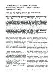
Figure 4.—Relationship between heterozygosity at 10 marker loci (each with H0 5 0.5) and phenotypic variance under additivity. The phenotypic variance is in units of s20, the phenotypic variance in the absence of inbreeding. DISCUSSION

Our aim was to derive the relationships between heterozygosity at neutral marker loci and the mean and variance of arbitrary phenotypes in infinite, partially inbred populations. In this section, I focus on three questions. First, how do the results on phenotypic means compare with and/or extend previous results? Second, what are the main conclusions regarding heterozygosityvariance relationships? Third, what is their relevance to empirical results? The relationship between heterozygosity and phenotypic mean in partially inbred populations: This model explicitly relates the phenotypic mean with fG, the average inbreeding level of a genotype. This relationship is linear, resulting in a simple prediction: whenever a trait is negatively affected by inbreeding (through overdominance, directional dominance, or both), phenotypic means at ML rank as heterozygote . common homozygote . rare homozygote. This has long been established by simulations (Charlesworth 1991; Pamilo and Palsson 1998) or analytically (Ohta and Cockerham 1974; Houle 1994), and has been repeatedly suggested as the probable origin of heterozygosity-fitness correlations (Houle 1989; David et al. 1997). However, alternatives, based on direct overdominance (see Mitton and Grant 1984) or multiple-locus dominance (Deng and Fu 1998), have also been cited. The occurrence of positive heterozygosity-fitness correlations, resulting from partial inbreeding, has indeed been referred to as a general effect (David et al. 1995), a special case of the associative overdominance hypothesis (Ohta 1971; Zouros 1993). The other case is the local effect arising from linkage disequilibrium in small populations (see David 1998 for review and definitions). This study extends previous results, providing a simple method (the computation of fG) to predict genotypephenotype relationships under partial inbreeding. Previous methods [Houle (1994), extended to multiple

Figure 5.—The change in mean (A) and variance (B) of a phenotype under dominance with increasing heterozygosity at 10 marker loci (each with H0 5 0.5). A is valid for arbitrary number, locus-specific effects, and allele frequencies of QTL. The phenotypic mean under random mating (φ0) has been arbitrarily set to 0 and the graphs are in units of R(2piqiai) (see Equation 23). B is represented for 100 QTL loci with identical effects on phenotype and allele frequency q 5 0.01. Graphs are in units of s20, the phenotypic variance under random mating. Range of s values as in Figure 4.

loci by David (1997)] relied on restrictive assumptions: small s and discrete inbreeding depression, neglecting the variance arising from the detailed genetic architecture of the trait. This study agrees with previous results, as the fitness predictors derived by Houle (1994; adaptive distances) and David (1997; g coefficients) are linearly related with fG in their domain of applicability. However, fG is more general, accounting for recurrent inbreeding and arbitrary genetic architecture. One of the predictions obtained using fG is that heterozygosity-phenotype relationships are nonlinear. They saturate because very heterozygous genotypes are almost exclusively outbred. Although intuitively predictable, this feature is usually ignored as most empirical studies use linear regressions. Of course, individuals with extreme MLH are rare and very likely lost from a sample of reasonable size. However, saturation at high MLH values is visually perceptible in some instances (Strauss 1986; David et al. 1997). The relationship between heterozygosity and pheno-

Heterozygosity and Variance

Figure 6.—Heterozygosity at 10 marker loci (each with H0 5 0.5) and phenotypic variance under symmetric overdominance for three numbers of overdominant QTL: (A) L 5 1; (B) L 5 10; and (C) L 5 100. Range of s values as in Figure 4.

typic variance in partially inbred populations: Until now, changes in phenotypic variance with inbreeding have been mostly envisaged in artificial, homogeneously inbred lines (Robertson 1952; Falconer and Mackay 1996). Recently, it has been recognized that the pattern of variation of mean and variance of fitness traits upon controlled inbreeding provides information on the underlying determinism such as selection coefficients and dominance (Deng 1998). This method was designed for either outcrossing or selfing populations at mutation-selection equilibrium. However, natural populations are often heterogeneous because of partial inbreeding. This generates genotype-phenotype correlations based on the distribution of genotypes among various inbreeding levels. These distributions determine phenotypic variances, because (i) inbreeding classes have different variances (within-class component), therefore genotypes concentrated in high-variance classes have higher variance and (ii) classes have different means (among-class component), therefore geno-

1469

types evenly distributed among classes have higher variance. The relative importance of (i) and (ii) depends on the genetic architecture. Very generally, heterozygotes appear to have lower variance than homozygotes in partially inbred populations. This applies to phenotypes coded by additive or directionally dominant alleles as well as by overdominant alleles in large regions of the parameter space including the most realistic situations. Additivity is expected for neutral phenotypes, directional dominance and/or overdominance being more common for fitness traits (Roff 1997). Negative heterozygosity-variance relationships have been predicted by Chakraborty (1987) in large, random-mating populations, but only when the marker genes themselves have additive effects on the phenotype (a quite unlikely situation). In nonrandom mating populations, negative heterozygosityvariance relationships have been predicted for fitness traits by David (1997) but with restrictive conditions (see above), and without evaluating the influence of the genetic architecture, the number of genes involved, and the inbreeding rate. The genetic architecture largely affects the relationships. Directional dominance results in large differences in variance among genotypes, one order of magnitude higher than the differences under overdominance, which in turn are larger than under additivity. Although details of genetic architecture are usually unknown, a broad consequence is that the influence of heterozygosity on variance will be larger for traits highly correlated with fitness (mostly under dominant or overdominant gene action) than for traits loosely or not correlated with fitness. The number of phenotype-coding loci (QTL) affects the relative importance of the within- vs. among-class components of variance. When many genes affect a trait, the stochastic variation in the overall sum of their effects is buffered, and all classes have low phenotypic variance. Increasing the number of QTL (L) thus reinforces the among-class component of variance compared to the within-class component [see (25) and (30)]. This effect is nonexistent under additivity (the among-class component is zero) and weak for dominant fitness traits [because of low frequencies of recessives—see (25)]. However, it is important under overdominance. Another consequence under overdominance is that when enough polymorphic marker loci are considered, the variance no longer decreases uniformly with heterozygosity. However, with an average scoring effort (10 polymorphic loci or less), this is perceptible only in largely inbred populations. Inbreeding rate also influences the patterns. When s increases, the decrease in variance with heterozygosity is steepened under additivity and dominance. However, under overdominance, increasing s rather tends to shift the maximum variance toward more heterozygous classes (Figure 6), although heterozygosity-variance relationships will be mostly negative for small s (,0.2–0.3).

1470

P. David

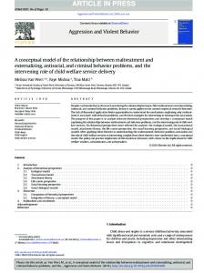
Moreover, the initial increase may be overlooked because very homozygous classes are often pooled together. Although higher s may yield variable outcomes, highly selfing species are rarely examined, being essentially devoid of heterozygosity and inbreeding depression (Charlesworth and Charlesworth 1987). The relevance of the model to empirical studies in natural populations: This study involves usual assumptions of quantitative genetics and inbreeding depression models. The assumption of homogeneity in locus-specific effects is unrealistic. However, mixtures of different determinisms have not been studied because of the number of situations to explore (Equation 10 provides a general formula). Negative heterozygosity-variance relationships are expected in mixed situations, because each determinism separately produces such relationships. The assumption of linkage equilibrium is not significantly violated in large populations, such as marine bivalves or trees (often used in empirical studies; cf. Britten 1996), even if QTL may be physically linked. The main difference between our model and actual situations lies with the environmental variance VE. The model considers only genetic variance, although all traits display various levels of nongenetic variation. VE will reduce relative changes in variance among genotypes, adding a constant to all. Furthermore, sampling variance must also be considered. Extreme heterozygosity classes have low sample sizes, hampering the estimation of phenotypic variance. A robust procedure is to pool extreme heterozygosity classes up to reasonable sample sizes (King 1985; David et al. 1997). Despite these potential problems, negative heterozygosity-variance relationships have been repeatedly observed in natural populations (see references in Introduction). Most of them have been interpreted as evidence for a direct role of enzyme heterozygosity in maintaining developmental stability without reference to a possible genetic variation of the traits. As shown by our model, partial inbreeding is a plausible alternative, especially for fitness traits. This is illustrated by a data set on heterozygosity at nine enzyme loci and growth in the bivalve Spisula ovalis (Figure 7, modified from David et al. 1997). Although the similarity between experimental and theoretical graphs obviously depends on an adequate choice of parameters, the observed pattern (shape of the heterozygosity-variance relationship, orders of magnitude) is consistent with the inbreeding hypothesis under dominance. In this instance, overdominance or additivity cannot generate effects of the observed magnitude. Although the redistribution of genetic variance upon inbreeding is sufficient to explain large changes in variance with MLH, developmental stability could also vary. Even if direct effects of allozymes on developmental stability might be negligible, inbreeding itself may influence developmental stability by increasing nongenetic variance (VE; Lerner 1954; Falconer and Mackay 1996). Effects of developmental stability and redis-

Figure 7.—Relationship between heterozygosity at nine allozyme loci and variance in growth, measured as t1/2, the age at half the maximum size in years, in the marine bivalve Spisula ovalis (see David et al. 1997). Classes MLH 5 0 and MLH 5 1 have been pooled to increase sample sizes. Error bars are 95% confidence intervals (slightly underestimated due to the nonnormality of distributions). The dotted line indicates theoretical predictions under partial inbreeding and directional dominance (Equation 25) with L 5 100 and q 5 0.01. A value of s 5 0.05 has been chosen because this species has separate sexes and natural levels of inbreeding must be small. The number of marker loci has been set to the observed value (9) and, for simplicity, all loci were assumed to have identical heterozygosity (Equations 31 and 32) equal to the geometric mean of observed values (geometric rather than arithmetic was used as heterozygosities interact multiplicatively rather than additively in Equations 31 and 32). The graph has been scaled to the observed values by setting s20 5 0.02.

tribution of genetic variance upon inbreeding are not easily distinguished. In practice, genotypic replicates, such as clonemates, are needed. Within-clone variance increased in inbred lines of the facultative parthenogens Daphnia pulex and D. pulicaria (Deng 1997), suggesting that inbreeding enhances developmental instability. Yet Yampolsky and Scheiner (1994) found no relationship between MLH and within-clone variance in D. magna, either because natural inbreeding is too low or because the results on pulex and pulicaria do not extend to magna. The two sides of a given individual are often used as substitutes for clonemates (e.g., Leary et al. 1983). However, the overall evidence for negative correlations between heterozygosity and fluctuating asymmetry appears weak (Britten 1996). In conclusion, partial inbreeding can generate MLH-variance relationships by two nonexclusive ways: altering developmental stability and redistributing genetic variance. The former relies on assumptions whose generality and quantitative importance remain to be properly established. The latter always occurs, and, in a variety of realistic situations, may produce detectable patterns qualitatively and quantitatively similar to empirical results obtained to date. I thank P. Jarne for helpful comments on the manuscript.

LITERATURE CITED Bamshad, M., M. H. Crawford, D. O. O’Rourke and L. B. Jorde, 1994 Biochemical heterozygosity and morphologic variation in a colony of Papio hamadryas hamadryas baboons. Evolution 48: 1211–1221.

Heterozygosity and Variance Bennett, J. H., and F. E. Binet, 1956 Association between mendelian factors with mixed selfing and random mating. Heredity 10: 51–56. Booth, C. L., D. S. Woodruff and S. J. Gould, 1990 Lack of significant associations between allozyme heterozygosity and phenotypic traits in the land snail Cerion. Evolution 44: 210–213. Britten, H. B., 1996 Meta-analyses of the association between multilocus heterozygosity and fitness. Evolution 50: 2158–2164. Chakraborty, R., 1987 Biochemical heterozygosity and phenotypic variability of polygenic traits. Heredity 59: 19–28. Chakraborty, R., and N. Ryman, 1983 Relationship of mean and variance of genotypic values with heterozygosity per individual in a natural population. Genetics 103: 149–152. Charlesworth, D., 1991 The apparent selection on neutral marker loci in partially inbreeding populations. Genet. Res. 57: 159–175. Charlesworth, D., and B. Charlesworth, 1987 Inbreeding depression and its evolutionary consequences. Annu. Rev. Ecol. Syst. 18: 237–268. David, P., 1997 Modeling the genetic basis of heterosis: tests of alternative hypotheses. Evolution 51: 1049–1057. David, P., 1998 Heterozygosity-fitness correlations: new perspectives on old problems. Heredity 80: 531–537. David, P., B. Delay, P. Berthou and P. Jarne, 1995 Alternative models for allozyme-associated heterosis in the marine bivalve Spisula ovalis. Genetics 139: 1719–1726. David, P., B. Delay and P. Jarne, 1997 Heterozygosity and growth in the marine bivalve Spisula ovalis: testing alternative hypotheses. Genet. Res. 70: 215–223. Deng, H.-W., 1997 Increase in developmental instability upon inbreeding in Daphnia. Heredity 78: 182–189. Deng, H.-W., 1998 Estimating within-locus nonadditive coefficient and discriminating dominance versus overdominance as the genetic cause of heterosis. Genetics 148: 2003–2014. Deng, H.-W., and Y.-X. Fu, 1998 Conditions for positive and negative correlations between fitness and heterozygosity in equilibrium populations. Genetics 148: 1433–1440. Eanes, W. F., 1978 Morphological variance and enzyme heterozygosity in the monarch butterfly. Nature 276: 263–264. Falconer, D. S., and T. F. C. Mackay, 1996 Introduction to Quantitative Genetics, Ed. 4. Longman, Harlow, United Kingdom. Gardner, J. P. A., 1995 Developmental stability is not disrupted by extensive hybridization and introgression among populations of the marine bivalve molluscs Mytilus edulis (L.) and M. galloprovincialis (Lmk.) from South-West England. Biol. J. Linn. Soc. 54: 71–86. Handford, P., 1980 Heterozygosity at enzyme loci and morphological variation. Nature 286: 261–262. Hartl, D. L., and A. G. Clark, 1997 Principles of Population Genetics. Sinauer Associates, Sunderland, MA. Hill, W. G., and A. Robertson, 1968 Linkage desequilibrium in finite populations. Theor. Appl. Genet. 38: 226–231. Houle, D., 1989 Allozyme-associated heterosis in Drosophila melanogaster. Genetics 123: 789–801. Houle, D., 1994 Adaptive distance and the genetic basis of heterosis. Evolution 48: 1410–1417. Kimura, M., and T. Ohta, 1971 Theoretical Aspects of Population Genetics. Princeton University Press, Princeton, NJ. King, D. P. F., 1985 Enzyme heterozygosity associated with anatomical character variance and growth in the herring (Clupea harengus L.). Heredity 54: 289–296. Leary, R. F., F. W. Allendorf and K. L. Knudsen, 1983 Developmental stability and enzyme heterozygosity in rainbow trout. Nature 301: 71–72. Lerner, I. M., 1954 Genetic Homeostasis. Oliver and Boyd, London. Livshits, G., and E. Kobyliansky, 1985 Lerner’s concept of developmental homeostasis and the problem of heterozygosity level in natural populations. Heredity 55: 341–353. Livshits, G., and P. E. Smouse, 1993 Relationship between fluctuating asymmetry, morphological modality and heterozygosity in an elderly Israeli population. Genetica 89: 155–166. McAndrew, B. J., R. D. Ward and J. A. Beardmore, 1982 Lack of relationship between morphological variance and enzyme heterozygosity in the plaice, Pleuronectes platessa. Heredity 48: 117–125. Mitton, J. B., 1978 Relationship between heterozygosity for enzyme loci and variation of morphological characters in natural populations. Nature 273: 661–662. Mitton, J. B., and M. C. Grant, 1984 Associations among protein

1471

heterozygosity, growth rate, and developmental homeostasis. Annu. Rev. Ecol. Syst. 15: 479–499. Mitton, J. B., and R. K. Koehn, 1985 Shell shape variation in the blue mussel, Mytilus edulis L. and its association with enzyme heterozygosity. J. Exp. Mar. Biol. Ecol. 90: 73–80. Ohta, T., 1971 Associative overdominance caused by linked detrimental mutations. Genet. Res. 18: 277–286. Ohta, T., and C. C. Cockerham, 1974 Detrimental genes with partial selfing and effects on a neutral locus. Genet. Res. 23: 191–200. Pamilo, P., and S. Palsson, 1998 Associative overdominance, heterozygosity and fitness. Heredity 81: 381–389. Robertson, A., 1952 The effect of inbreeding on the variation due to recessive genes. Genetics 37: 189–207. Roff, D. A., 1997 Evolutionary Quantitative Genetics. Chapman & Hall, London. Smouse, P. E., 1986 The fitness consequences of multiple-locus heterozygosity under the multiplicative overdominance and inbreeding depression models. Evolution 40: 946–957. Strauss, S. H., 1986 Heterosis at allozyme loci under inbreeding and crossbreeding in Pinus attenuata. Genetics 113: 115–134. Strobeck, C., 1979 Partial selfing and linkage: the effect of a heterotic locus on a neutral locus. Genetics 92: 305–315. Weir, B. S., and C. C. Cockerham, 1973 Mixed self and random mating at two loci. Genet. Res. 21: 247–262. Yampolsky, L. Y., and S. M. Scheiner, 1994 Developmental noise, phenotypic plasticity, and allozyme heterozygosity in Daphnia. Evolution 48: 1715–1722. Yezerinac, S. H., S. C. Lougheed and P. Handford, 1992 Morphological variability and enzyme heterozygosity. Individual and population level correlations. Evolution 46: 1959–1964. Zink, R. M., M. F. Smith and J. L. Patton, 1985 Associations between heterozygosity and morphological variance. J. Hered. 76: 415–420. Zouros, E., 1993 Associative overdominance: evaluating the effects of inbreeding and linkage desequilibrium. Genetica 89: 35–46. Zouros, E., S. M. Singh and H. E. Miles, 1980 Growth rate in oysters: an overdominant phenotype and its possible explanations. Evolution 34: 856–867. Communicating editor: P. D. Keightley

APPENDIX A: APPROXIMATIVE DISTRIBUTION OF INBREEDING LEVELS WITH SELECTION

Without selection, inbreeding classes 0, 1, . . . , k have frequencies (1 2 s), s(1 2 s), . . . , sk(1 2 s). However, mean fitness wk usually decreases when inbreeding (k) increases. Therefore the equilibrium distribution of k has lower frequencies of inbred classes (k . 0) than the neutral distribution. Therefore, the effect of selection resembles a decrease in selfing rate s to a lower value s9. Let us compute s9 values that provide reasonably accurate distributions of k. Let the frequency of class k be lk. Assuming w0 5 1, the change in the lk’s during one generation is

12 1 l0 l1 … lk …

1 5 wt

t11

(1 2 s) (1 2 s) … (1 2 s) (1 2 s) sw1 0 0 0 0 0 … 0 0 0 0 0 swk 0 0 0 0 0 … 0

212 ·

l0 l1 … , lk … t

(A1) or more concisely, Lt11 5

1 S · L t, wt

(A2)

where wt is the mean fitness at time t. The population eventually reaches a steady state, the increase in k through selfing being exactly compensated by selective

1472

P. David

elimination of inbred individuals. The equilibrium mean fitness w∞ is the real eigenvalue of S and the distribution of k at equilibrium is the corresponding unitary eigenvector L∞. Although w∞ cannot be computed analytically, numerical values can be obtained, restricting S to a reasonable dimension (say, kmax 5 10) and setting values to the wk’s according to a selection model. L∞ can then be computed using lk,∞ 5 ((1 2 s)sk/w k∞11) pkj50wj. The approximation should conserve the crucial characteristics of the distribution of k for heterozygosityvariance relationships, i.e., the mean and variance of fk. The former is f∞ 5 R∞k50lk,∞(1 2 1/2k) at equilibrium. We need only the first few terms for numerical estimations. As the approximate distribution of k is constructed as the neutral distribution under a selfing rate s9, its mean f is the classical s9/(2 2 s9). This will be equal to the true f∞ provided s9 5 2f∞/(1 1 f∞). The accuracy of this approximation was tested under a simple multiplicative selection model: wk 5 (1 2 a)fk (0 , a , 1). s9 was determined numerically as explained above for a variety of s (0.05–0.8) and a (0–1) values. Stronger inbreeding depression (a z 1) generates larger reduction (s9 , s) in apparent inbreeding, although the absolute value of s has little influence on this reduction (data not shown). The variance and third central moment of f for the approximate distribution are compared to their numerical values under selection in Table A1. The approximate distribution is generally very close to the actual one. The largest discrepancy is obtained in an unlikely situation (high inbreeding depression and high selfing rate).

APPENDIX B: THE CHANGE IN ALLELIC FREQUENCIES AND HOMOZYGOSITY OF A DELETERIOUS ALLELE WITH INBREEDING UNDER PURGING SELECTION

Consider a single locus with two alleles A, B of respective zygotic frequencies p, q in the population, and p(k),

q(k) in inbreeding class k. The deficiency in heterozygous (AB) genotypes within class k compared to randommating expectations is noted f(k). Without selection, q(k) 5 q for all k, and f(k) 5 1 2 1/2k. However, if the fitnesses of AA, AB, BB are 1, 1, 1 2 z, respectively, and ignoring mutation, q(k) and f(k) change from class (k) to class (k 1 1) (one generation of selection followed by selfing), q(k 1 1) 5

q(k) 2 1 1 w(k) w(k)

f(k 1 1) 5 1 2 [1 2 f(k)]

(B1)

q(k) , 2q(k 1 1)

where w(k) 5 1 2 z[q(k)2 1 f(k)p(k)q(k)] is the mean fitness of class k. As expected, q(k) decreases when k increases, and selection slows down the increase in f(k). Although recurrent mutation must exist to maintain the B allele, it only tends to restore neutral frequencies. Therefore, ignoring mutation leads only to overestimation of purging effects. Plugging (B1) and (B2) into (4) and (5) does not yield a simple expression of phenotypic mean and variance within class k. I therefore obtained numerical estimates (iterating B1 and B2) and compared them to neutral predictions. The expected homozygote-to-het2 2 erozygote ratio of phenotypic variances (shom /shet ) was calculated numerically (neglecting inbreeding classes with k . 25) with and without selection. P was set at 0.5 and q at 0.01. All combinations of three s (0.05, 0.1, 0.3) and three z (0.05, 0.1, 0.3) values were considered. The simulations without selection perfectly matched analytical predictions (Equation 25). Selection reduced 2 2 /shet ) by an amount ranging from 0.2% the ratio (shom (s 5 0.05, z 5 0.05) to a maximum of 8.3% (s 5 0.3, z 5 0.3, an unlikely situation). The same parameter combinations were tested with several QTL (L 5 10 and 100) in linkage equilibrium, and the effect of selec2 2 tion on (shom /shet ) always remained within the same range (0 to 28.5%). Therefore purging selection does

TABLE A1 Comparison of the variance and third central moment of f between the actual situation (inbreeding s and selection a) and the approximation (inbreeding s9, no selection) s: a: s9 f∞ s2( f )actual s2( f )approx. Third central moment, actual Third central moment, approx.

(B2)

0.1 0.9

0.1 0.5

0.5 0.9

0.5 0.5

0.0332 0.0169 0.0083 0.0084 0.0039 0.0041

0.0716 0.0372 0.0181 0.0182 0.0083 0.0085

0.2118 0.1185 0.0512 0.0551 0.0174 0.0213

0.3855 0.2387 0.0958 0.1006 0.0217 0.0252

The mean f over all inbreeding classes, noted f∞, is by construction the same for both situations. Numerical estimates for f∞, variances, and third moments have been taken to the order k 5 15.

Heterozygosity and Variance

not considerably affect heterozygosity-variance relationships. APPENDIX C: THE CHANGE IN HOMOZYGOSITY AT SYMMETRICALLY OVERDOMINANT LOCI WITH INBREEDING

Allele frequencies at symmetrically overdominant loci are p 5 q 5 1⁄2, irrespective of inbreeding. Without selection, heterozygosity is halved following every generation of selfing. Under overdominance, the decrease in heterozygosity will be slower as heterozygotes have higher viability than homozygotes (say, 1 1 z for genotype AB and 1 for AA and BB), f(k 1 1) 5 1 2

[1 2 f(k)](1 1 z) , 2w(k)

(C1)

APPENDIX D: THE EFFECT OF PHYSICAL LINKAGE

Physical linkage increases identity disequilibria in selfed lineages (Charlesworth 1991), although it does not generate linkage disequilibria in infinite populations. Two cases are envisaged: (1) linkage among QTL and (2) linkage between ML and QTL. 1. Heterozygosities at linked QTL are correlated within a given inbreeding class. Consequently, phenotypic contributions of loci i and j covary within class k by an amount (D1)

The identity disequilibrium hijk depends on inbreeding (k) and linkage lij (5 1 minus twice the recombination fraction between i and j):

1

2 12

1 1 lij2 k 1k hijk 5 2 4 4

additively. Thus, relationships between genotypes and phenotypic means [(4) and (9)] stay unchanged, provided ML and QTL remain unlinked. Charlesworth (1991) predicted slight differences (a few percent) in associative overdominance between unlinked and completely linked (l 5 1) QTL, probably because QTL effects were considered multiplicative instead of additive and purging selection was not neglected. Linkage among QTL affects the withinclass component of variance more seriously, sG2 (linked) 5 sG2 (unlinked)

(D2)

(Weir and Cockerham 1973). Covariation of QTL effects does not affect class means when QTL interact

(D3)

1 8oopipjqiqjdidjhij,G , i j .i

where hij,G 5

where w(k) 5 1 1 z[1 2 f (k)]/2 and f(k) is the zygotic heterozygote deficiency within class k. As in appendix b, numerical simulations (up to k 5 25) were used to estimate the influence of selection as (C1) does not 2 2 /shet ). Simulations yield a tractable expression of (shom using (C1) and parallel simulations using neutral f distributions were performed for all combinations of three s (0.05, 0.1, 0.3) and z (0.05, 0.1, 0.3) values, using 1, 2, 5, 10, and 50 QTL and P 5 0.5. The neutral simulations perfectly matched analytical predictions from (30). The other results (not shown) indicate that (30) tends to exaggerate absolute changes in variance between het2 2 erozygotes and homozygotes. Thus, (shom /shet ) is underestimated when ,1 (one QTL) and is overestimated when .1 (several QTL). However, the effect of selection 2 2 /shet ) is always small (from 11.3% for L 5 1, on (shom s 5 0.3, z 5 0.3; to 26.5% for L 5 50, s 5 0.1, z 5 0.3).

Covk(φi,φj) 5 4pipjqiqjdidjhijk.

1473

ok Gkhijk

(D4)

and sG2 (unlinked) is given by (10). From D3, linkage among QTL has no effect on purely additive phenotypes (di 5 0). However, it does affect heterozygosity-variance relationships under directional dominance or overdominance. The exact expressions for the hij,G’s, obtained from D4, D2, 11, and 12, are complicated. First-order approximations are hij,Mm 5 lij2s/8 1 0(s2)

(D5)

and hij,MM 5 [(2 2 Q)/(1 2 Q)]lij2s/8 1 0(s2). (D6) Therefore, hij,G is positive and more than twice as large in homozygotes than in heterozygotes. It will increase the difference between them. For fitness traits under directional dominance, this increase may be negligible as qi and qj are small. However, under overdominance, with several QTL, the variance is mainly sensitive to sf2(G), which is of order s/8. Therefore, tight linkage among QTL (lij ≈ 1) may appreciably increase the negative heterozygosity-variance correlation. 2. I now consider linkage between ML and QTL. Consider an indicator variable IG, which equals 1 for individuals of genotype G and 0 otherwise. Because of physical linkage, IG and phenotypic values covary within class k. This is quantified by two parameters, aG,k 5 covk(IG,φ)/p(G|k) and bG,k 5 covk(IG,φ2)/p(G|k), where covk means the covariance and p(G|k) the frequency of G within class k. Introducing covariance terms into (6) and (7) yields φG 5 φG,unl 1 aG

(D7)

2 (φ) 1 bG 1 aG2 2 2aGφG, sG2 (φ) 5 sG,unl

(D8)

and

where unl denotes values for an unlinked ML (Equa-

1474

P. David

tions 6 and 7), aG 5 RkGkaG,k , and bG 5 RkGkbG,k. For a single QTL, we obtain aMm 5

4pqd(2 2 s)sl2 (4 2 s)[4 2 s(1 1 l2)]

(D9)

and bMm 5 daMm ,

(D10)

l being the linkage between the ML and the QTL. Values for pooled homozygotes (MM 1 mm) are identical except for an opposite sign for a. Heterozygosity-mean and heterozygosity-variance relation-

ships are not affected when the phenotype is additive (d 5 0). However, under dominance, the average phenotypic difference between heterozygotes and homozygotes increases. For small s and P 5 Q 5 1⁄2, the increase is approximately proportional to (1 1 l2) (always ,2), as in Charlesworth’s (1991) numerical results. Similar effects are observed under overdominance. Moreover, under dominance or overdominance, linkage also increases differences in variance between heterozygotes and homozygotes (the last term of D8 being negative for the former and positive for the latter).