A Query Processing Model for Mobile Computing using Concept Hierarchies and Summary Databases Sanjay Kumar Madria
Mukesh Mohania and John F. Roddick
Centre of Advanced Information Systems Faculty of Applied Science Nanyang Technological University Singapore
Advanced Computing Research Centre Faculty of Computer and Information Science University of South Australia The Levels Campus, Mawson Lakes, Adelaide, South Australia 5095
[email protected] {mohania, roddick}@cis.unisa.edu.au
Abstract We present a query-processing model for mobile computing using summary databases (database stored in some predefined condensed form). We use concept hierarchies to generate summary databases from the main database in various ways. Traditional database management systems are correct in that they are able to provide answers to queries that are both sound and complete with respect to the source data. In a mobile environment, it may be advantageous to relax one or other of these criteria to enhance availability through the use of summary databases. This would provide a more optimal use of data during periods of disconnection and to enable efficient utilization of low bandwidth and restricted memory size. The model for query processing proposed uses concept hierarchies and summary databases at run time to return approximate queries when access to the main database is either undesirable or unavailable. We present a model that is able to provide varying levels of approximate answer to queries that occur at a mobile host using the summary database stored either locally at mobile host (MH) or remotely at mobile service stations (MSS). The paper also discusses some cost-benefit analyses involving storage, transmission and query processing costs. Keywords – query processing, mobile computing, summary database, concept hierarchy, sound, complete.
1
Introduction
Traditional database systems have been designed to provide correct (i.e. sound and complete) answers for database queries. It is clear that for many emerging environments such as wireless computing it is neither practical nor necessary to adhere to such a stringent requirement. In a mobile computing environment, characteristics such as availability, connectivity, low-band width, data quality, usage cost and query imprecision impose new constraints on database systems [IB1, PB, MM]. In such a computing environment, users may not obtain perfect answers to their queries within an acceptable time. However, within known limits of correctness and precision, an approximate answer may suffice for some mobile users [BDW]. For these reasons, much recent database research on query processing [IB2, TGNO, AG] is focused on exploring the techniques for providing approximate or incomplete answers in various environments [HHW, FJS, ABF+, GM, VL, R]. In wireless computing, caching of frequently accessed data items is an important technique that reduces contention on a small bandwidth wireless network [E]. This technique aims to improve query response time and to support disconnected or weakly connected operations [KS]. If a mobile user has cached a portion of the shared database, different levels of consistency may be requested. During times of strong connection with the main database server at MSS, a user is in a position to request the current values of the database, whereas during weak connections, a user may allow a weaker level of correctness where the cached copy may be used as a surrogate (and smaller) replica of the central database. Each type of connection may have a different degree of allowable consistency associated with it.
1
Due to the expense and complexity of maintaining replicated data [BI], mobile database systems must limit the amount of replication or cached data items. Since data is not fully replicated, it is possible to pose only a limited set of queries during a disconnection in which main database is not available. Queries that require the main database are typically either delayed until the connection is established or are aborted with some explanation to the user. In short, query processing in mobile computing environments becomes difficult at times of weak connection or disconnection and we thus contend that in these circumstances, queries may be answered in an approximate way to increase availability. Given a query, the mobile host may optimize the cost by determining whether it can process the query using cached data or transmit a request for data to the mobile service station. The task is thus to construct a summary database and a query processing system which can maximize its use in a mobile computing environment. We argue here that in environments such as these it may not be necessary to provide both accurate and exhaustive answers to queries [R, RCR1]. Due to the limitations of memory and computing power, it is reasonable to answer queries using a condensed form of the main database, which we term in this paper a summary database. Summary databases are typically orders of magnitude smaller than the main database, and hence can more easily be stored on the mobile host. During disconnection or weak connections, five strategies can be employed: •
The query can be denied;
•
The query can be stalled until a better connection is available;
•
During weak connection, the limited bandwidth can be used to answer the full question resulting in longer response times;
•
Summary data can be used to reply to the queries posed by mobile users, which may result in an approximate answer. This can be verified (if needed) by accessing the main database during periods of strong connection;
•
Finally, the query processor at mobile host may decide to rephrase the query to use only summary data to get an answer to an alternative query.
In this paper, we are interested in the last two strategies listed above. To summarize the main database, we make use of concept hierarchies [HCC, HHCF, R, RR]. Concept hierarchies are generally supplied a priori by the DBA but can also be generated from the domain information available about the attributes and on the functional dependencies that exist in a particular relation. We propose several ways of summarizing the database using concept hierarchies. We map queries to appropriate summary data and concept hierarchies to answer the queries that may yield “sound but not complete” approximate answers [R, RCR1]. We have also discussed the cost-benefit analysis with respect to storage, communication and query processing cost. Our query-processing model is different from the model proposed by Han et al. [HHCF]. The model proposed in [HHCF] for intelligent query processing uses concept hierarchies, however, the queries are rewritten using lower level concepts. Our model uses higher level concepts, thus providing approximate answers possibly in fewer steps. More importantly, we have proposed methods for summarizing a database. We categorize both the database and the returned response based on a set of correctness properties and we have included a cost-benefit analysis of our model when used in a mobile environment.
2
Mobile Query Processor Architecture and Modes of Operations
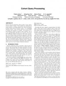
In mobile computing environments (see Figure 1), the network consists of stationary and mobile hosts [M]. A mobile host (MH) can change its location and network connections while computations are being processed. While in motion, a mobile host retains its network connections through the support of stationary hosts with wireless connections. These stationary hosts are called mobile support stations (MSS) or base stations. Each MSS is responsible for all the mobile hosts within a given small geographical area, known as a cell. At any given instant, a MH communicates only with the MSS responsible for its cell. A MH has some server capability to perform computations locally. In Figure 1, both the MSS and MH have a query processor (QP) and summary databases (SDB), while MSS also has main databases (DB). Thus, a mobile host can process the query using summary data and return an approximate result whereas MSS can return an exact or approximate answer.
2
When a MH leaves a cell serviced by a MSS, a hand-over protocol is used to transfer the responsibility for a mobile transaction and data support to the MSS of the new cell. This hand-off involves establishing a new communication link. It may also involve migration of in-progress transactions and database states from one MSS to another. In mobile computing, there are several possible modes of operations [PB]. The operation mode in mobile computing may be one of the following: •
fully connected (normal connection)
•
totally disconnected (MH may be out of range of all MSS)
•
partially connected or weak connection (a terminal is connected to the rest of the network via low bandwidth).
These disconnected modes should be expected in mobile computing and a mobile host should be able to operate autonomously even during total disconnection. A disconnection protocol is executed before the mobile host is physically detached from the network. The protocol should ensure that enough information is locally available (cached at the mobile host) for its autonomous operation during disconnection. A partially-disconnection protocol prepares the mobile host for operation in a mode where communication with the fixed network is restricted. Selective caching of data at the host site will minimize the future network use.
Fixed Network
MSS1
MSS2 QP
SDB
MSS3 QP
DB
SDB
QP
DB
SDB
DB
MH QP
SDB
Figure 1 – Architecture of a Mobile Database Environment
3 3.1
Classifications of Databases and Query Responses Classification by Correctness
In this section, we first classify databases based on the “correctness” of information they contain with respect to the main database. We also classify the types of response returned.
3
Consider a database S that stores some part (or summary) of a larger database T and assume that both S and T are relational databases. We will consider database T as the main database and S as its approximation (which we call a summary database). We formalize some definitions as follows: Definition 1: S is complete with respect to T if S “contains” T. That is, all information stored in S includes all the information that is contained in T. Definition 2: S is sound with respect to T if S is “contained in” T. That is, the stored information in S includes only true information that stored in T. Definition 3: S is imprecise with respect to T when it contains an approximation with respect to the values held in T. For example, S may contain a set of possible values, with the real value (held in T) being one of the elements of this set. Imprecise information is not erroneous and does not necessarily compromise the integrity of an information system. These three definitions can also be redefined in terms of the responses to queries: Definition 1B: S is complete with respect to T if a query on S will return at least the data that the same query would return on T. Definition 2B: S is sound with respect to T if a query on S will return no additional data than would the same query on T. Definition 3B: S is imprecise with respect to T if a query on S contains values that are either numerically approximate or conceptually broader. We are now in a position to define a summary database. Definition 4: A summary database S is a special form of information repository in which data are stored in a condensed or summarised form. Summary databases are generally, by their nature, incomplete but sound and may be imprecise. 3.2
Inaccuracy and Summary databases
Suppose τ ={t1, t2….. tn} is the set of tuples that satisfy a relational query on the database T and γ = { r1, r2….. rn} is the set of tuples which are actually returned using S. An answer returned, for the purpose required here, can be classified as follows: 1. Correct and complete, i.e., γ = τ. 2. Potentially understated (i.e., sound but may be incomplete) i.e., ∀r ∈ γ : r ∈ τ. 3. Potentially overstated (complete, but may not be sound) i.e., ∀r ∈ γ : r ∈ τ ∨ r ∉ S and ¬∃t ∈ τ : t ∉ γ. 4. Wrong, i.e., ∃ r ∈ γ : r ∉ τ ∧ r ∈ S. The difference between 1 and 3 lies in the relaxation of the closed world assumption that anything not recorded in the database may be assumed false. Potentially overstated responses are correct as far as there is no evidence recorded to the contrary.
4
Concept Hierarchies
Concept hierarchies define a sequence of mappings from a set of lower-level concepts to their higher level correspondences [HCC, RCR1, R] resulting in a hierarchy of concepts. In other words, concept hierarchies provide a set of predefined hierarchical relationships that generalize lower layer (i.e., primitive data) information to high layer ones. For example, a set {tennis, rugby, hockey, football} can be generalized as “sports” at a high level concept. A concept hierarchy can be defined on one or on a set of attribute domains. Suppose a hierarchy H is defined on a set of domains D1,…,DKr, in which different levels of concepts are 4
organized into a tree or lattice structure. The most general concept is the “all” description (described in general by the term “any”) whereas the most specific concepts correspond to the specific values of attributes in the database. The concept hierarchies in general are data or application specific since they define mapping rules between different levels of concepts. The mapping of a concept hierarchy or some portion of it may also be provided explicitly by a knowledge engineer or a domain expert. Many different concept hierarchies can be constructed based on different view points or users preferences. However, usually, a common concept hierarchy can be associated with an attribute. In most database system implementations, it would be possible for a set of relatively stable and standard concept hierarchies to be made available as a common reference by all the databases. In [HF], an automatic and dynamic generation of concept hierarchies is given. Our work is delimited as follows: •
We consider only set-valued domains of an attribute although we believe that the method is also appropriate for continuous domains, and therefore suitable for numeric data.
•
We also assume that set-valued domains of attributes are simple structure-valued domains containing only discrete values. These set-valued domains can be generalized into a high level concept, which we call a super-domain.
•
We summarize our relational databases by summarizing the attribute’s values using higher or lower level concepts. For simplicity in our discussion, as far as possible, we consider each concept hierarchy to consist of only two levels of nesting. However, in general, a concept hierarchy can have any level of depth.
Concept hierarchies can be generated among attribute domains for the following: •
Within a domain itself, there may exist a concept hierarchy among the values. For example, a domain may be successively refined into more specialised domain values. An attribute may take its value either from the specialised (leaf) values or from higher level descriptions.
•
A concept hierarchy can be defined among attributes using domains of attributes of a relation. For example, attributes “Department” and “Faculty” can be related by a concept hierarchy with “Faculty” at the root (since a Faculty can have many departments) and “Department” at the leaf level. Here we assume that each Faculty has many Departments.
•
There may exist a concept hierarchy among domains of attributes of different relations. For example, consider attributes “Department” and “Faculty” which may appear in two different relations. In that case, we can define a concept hierarchy across these two tables where “Faculty” appears at higher level and “Department” at lower level. Definition 5: A summary database system (SDS) is constructed using two major components (T, H) which are as follows: T - main database consisting of relations; H - a set of pre-defined or dynamically generated concept hierarchies within and among relations in the database.
4.1
Construction of Concept Hierarchies
Concept hierarchies are constructed as part of the database definition phase for each of the attributes across all relations by constructing a classification hierarchy based on the domain values of those attributes. Domain experts can be consulted to ensure that the hierarchies are complete and correct. Thus, the concept hierarchies of domain values are static. Note that since we are constructing the concept hierarchies based on domain values, there is no need to incrementally update such hierarchies when: •
new values are inserted in the relation.
•
values are deleted from the relation. 5
•
new relations are introduced in the database.
Concept hierarchies need change only when domains are changed by insertion or deletion. There is also no need to send the updated concept hierarchies from MSS to MH except in cases where there is an update to the definition of the database. This will save much of wireless transmission cost. However, we need some extra storage at mobile host, particularly in cases where the concept hierarchies are large. Note that one may construct concept hierarchies involving only instances of domain values that occur in a given table. In that case, one may have to update concept hierarchies. Also, since many attributes may draw their values from a common domain, there is no need to construct concept hierarchies of instances based on different tables, which otherwise needs extra storage. 4.2
Key Alteration
Generalizing attributes using a concept hierarchy may result in the loss of the key or foreign key information as generalization may remove or alter the key or foreign key values of a relation. Thus, the generalized key should be marked explicitly since they usually can not be used as join attributes. It is therefore crucial to find altered keys since if the altered keys were used as join attributes for joining different relations, it may generate erroneous information. Two types of generalizations are possible as follows. •
Key-preserving generalization, in which all key or foreign key values or attributes are preserved.
•
Key-altering generalization, in which some key or foreign key values or attributes are generalized, and thus, altered.
5
Generating Summary Database using Concept Hierarchy
In this section, we first define some terminology that will be used later in our discussion. We then illustrate various ways of summarizing a relation using examples and discuss examples of summarizing a relation. Finally, we give algorithms for each types of summarization. 5.1
Some definitions
Consider a relation schema R (A1, A2,…An) is composed of a relation name R and a list of attributes Ai. Each attribute is the name in that relation of a role played by some domain D in the relation schema R. Di is the domain of attribute Ai. Formally: Definition 6 : A relation r(R) is defined as a sub-set of the Cartesian product of the domains that are in the schema R: r(R) ⊆ (dom (A1) × dom(A2) ×…., × dom(An)). A given element is a tuple t of a cross product of values from the underlying domains and denoted as t = [v1, v2,….,vn] where each value vI is an element of dom(Ai). Next, we need to relate tuples via defining a sub-set, sub-type or super-type as follows: Definition 7A : A tuple ta = [v1, v2,…,vi] of ra(Ra) ⊆ (dom (A1) × dom(A2) ×…, × dom(Ai)) is a sub-set of another tuple tb = [v1, v2,…, vj] of rb(Rb) ⊆ (dom (B1) × dom(B2) ×…, × dom(Bj)) if [v1, v2,…,vi] ⊆ [v1, v2,…, vj] where each vi is an element of dom(Ai ) and each vj is an element of dom(Bj). Definition 7B : A tuple ta = [v1, v2,…,vi-1] of ra(Ra) ⊆ (dom (A1) × dom(A2) ×…, × dom(Ai-1)) is a sub-type-1 of another tuple tb = [v1, v2,…,vi] of ra(Ra) ⊆ (dom (A1) × dom(A2) ×…, × dom(Ai)) if there exists a concept hierarchy from the dom(Ai-1) to dom(Ai). We can call tb = [v1, v2,…,vi] also a super-type-1 of tuple ta = [v1, v2,…,vi-1]. Definition 7C : A tuple ta = [v1, v2,…, vi] of ra(Ra) ⊆ (dom (A1) × dom(A2) ×…, × dom(Ai)) is a sub-type-2 of another tuple ta = [V1, V2,…,Vi] of S(ra(Ra)) ⊆ (super dom (A1) × super dom(A2) ×…, × super dom(Ai)) where S(ra(Ra)) is the summarized relation if there exists a concept hierarchy from [V1, V2,…,Vi] to [v1, v2,…, vi] where each vi is an element of dom(Ai) but each Vi ∈ super dom (Ai) (i.e., if Vi is at root 6
level in the concept hierarchy then vi is at sub-concept level (child level). Vice-versa, We can call tuple ta = [V1, V2,…,Vi] to be a super-type-2 of tuple ta = [v1, v2,…,vi-1]. Definition 7D : A tuple ta = [v1, v2,…,vi] of ra(Ra) ⊆ (dom (A1) × dom(A2) ×…, × dom(Ai)) is a sub-type-3 of another tuple tb = [v1, v2,…, vj] of rb(Rb) ⊆ (dom (B1) × dom(B2) ×…, × dom(Bj)) if there exists a concept hierarchy from [v1, v2,…,vi] to [v1, v2,…, vj] each vi is an element of dom(Ai ) and each vj is an element of dom(Bj). 5.2 •
Types of Summarization Horizontal Summarization This involves summarising a relation using the concept relationships between attributes. In this case, we identify the concept hierarchies involving attributes in a single relational table. We have two options. In first case, we project out the attribute(s) which occur at lower level in the concept hierarchy. In second case, we project out the attributes that occur at higher level. Condensing a relation by projecting out attributes results in the relation size to be reduced horizontally. That is, the number of attributes will be reduced. Note that it duplicate tuples might be created and in this case the relation can be further condensed by eliminating duplicate tuples.
•
Vertical Summarization This involves summarising tuples using higher-level domain knowledge in the concept hierarchy. Here, we first identify the cases where tuple values occur at lower level in the concept hierarchies. The higher level concepts need not belong to the domain sets but may belong to super domain of those sets. We replace the group of tuple values that occur at lower level in the concept hierarchy by their higher level counter parts and duplicate tuples are removed. In this case, the relation can be summarized vertically.
Consider the following relational schema for faculty database at a typical University in which staff are located in Departments which are in turn located within Faculties. The domain set of “Faculty” will contain the values able to be held by that attribute (eg. dom(Faculty) = {Science, Engineering, Arts, Education}). Each Faculty has Departments and thus the Faculty domain can be further subdivided [RR] and a full domain definition might be as follows: DOM(FACULTY) = {Science = {Mathematics, Chemistry, Computing, Physics}, Engineering = {Civil, Mechanical, Electrical, Electronic}, Arts = {Visual, Performing, Literary}, Education = {Primary, Secondary}, Humanities = {History, Social Science} … etc. Each faculty member belongs to one of the “Faculty”, and further belongs to one of the “Department”. For example, in Faculty of Science, each faculty member is associated with one of the Departments Science such as the Department of Mathematics, etc. Name
Faculty
Department
Sanjay
Science
Mathematics
Anil
Science
Computing
Murli
Science
Mathematics
John
Arts
Literary Arts
Mukesh
Engineering
Electronic Engineering
Fredric
Education
Secondary Education
Table 1 - Example Faculty-data Relation Now consider the faculty-data relation given in Table 1. In faculty-data, there is a dependency Department → Faculty; each Department belongs to one Faculty only. That is, when the Department name is same, Faculty name will be same. Note that knowledge of the existence of this dependency may be for two reasons:
7
•
A known characteristic due to existence of the functional dependency and therefore known by the DBA during database construction. In this case, the Faculty-data relation contravenes 3NF and is presumably deliberately unnormalised.
•
A coincidence of the data currently held in the relation and has been found through some mining process (i.e., an induced dependency [RCR2]). In this case, any later updates to the relation may break this dependency and the update frequency may determine whether summarization is worthwhile.
Note that given domain and functional dependency knowledge, the concept hierarchies can be generated if they are not supplied by the DBA. There are two broad types of concept hierarchy: Inter-Attribute Hierarchies (IAH) in which a functional, induced dependency or some other known relationship between two attributes is used (see left-hand side of Figure 2) and Domain Values Hierarchies (DVH) in which domain values are used (see right-hand side of Figure 2). While they can be generated from the same data – they are independent. A DVH can exist for (a subset of) the domain values without any IAH being possible. Moreover, an IAH may be recorded without a DVH being held. IAH
DVH
Faculty
Science
Engineering
etc... Department
Mathematics
Computing
Chemistry
Physics
Civil
Mechanical
Electronic
Figure 2 - Concept Hierarchies of (a) Attribute Dependencies and (b) Domain Values 5.3
Summarising a Relation by Applying the Inter-Attribute Hierarchies
The relation in Table 1 can be summarized using these concept hierarchies in many ways. Case 1- Table 1 is condensed by projecting out the attribute “Department” since Department is a sub-type-1 of the higher level concept “Faculty” as shown in Figure 2. Thus, the resulting table will have only two attributes. This summarized table is incomplete, sound and imprecise; it contains only true information and represents a subset of the information (in the sense of tuple values) in comparison to the original facultydata in Table 1. Each tuple involving the attribute “Faculty” in the summarized table represents a supertype-1 tuple value for the corresponding projected out attribute “Department”. Thus, in general, the summarized table represents a super-type-1 of information in the sense of the concept hierarchy involving “Faculty” and “Department”. Name
Faculty
Sanjay
Science
Anil
Science
Murli
Science
John
Arts
Mukesh
Engineering
Fredric
Education
Table 2 - Summarized Faculty-data relation Suppose that a Department belongs to two Faculties. That is, the dependency, Department → Faculty, does not hold. In this case, the concept hierarchy shown in Figure 2 will not exist and concept hierarchy involving only two levels become lattice-structured rather than tree-structured. In this paper, we will not elaborate much on this in our discussion, as we are restricting ourselves with the concept hierarchy with only two levels nesting. However, it should be noted that a DVH can still be built for static data and that induced dependencies may exists for selections of the relation. Now we give the algorithm in Pseudo-code: 8
Algorithm 1: Construction of a Summary table (case1) Input – a relational table and a set of predefined concept hierarchies. Output – A summarized table. Method – 1.
search the given concept hierarchies for any two attributes of a given relation
2.
If a concept hierarchy is found which relates any two attributes of the relation then
•
project out the attribute from the relation which occurs at lower level in the concept hierarchy;
•
Repeat 1 for all the pairs of attributes; else the relation can not be summarized.
3.
Remove duplicate tuples if any.
Case 2 – The table is summarised by removing the attribute “Faculty” which occurs at higher level in the concept hierarchy shown in Figure 2. Thus, the resulting table will have the two attributes “Name” and “Department”. The summarized Table 3 will be sound, complete and precise. That is, if a CHDV has been built and stored, the summary table contains all the information that was contained in the original facultydata table and the original table can be recreated. However, in this case, attribute “Department” represents a sub-type-1 of attribute “Faculty”. The algorithm is similar to case 1 and therefore, is not reproduced here. Name
Department
Sanjay
Mathematics
Anil
Computing
Murli
Mathematics
John
Literary Arts
Mukesh
Electronic Engineering
Fredric
Secondary Education
Table 3 - Summarized Faculty-data Relation 5.4
Summarising a Relation using Domain Value Hierarchies
Case 3 - Consider the following relation Sub-dept (subject, department) as shown in Table 4 where: Dom(Subject) = {Database Systems, Information Systems, Compiler, Material Science, Physical Chemistry, Organic Chemistry, Atomic Physics, Nuclear Physics, Literature, Drama}. The concept hierarchy for the attributes “Subject” (given below in Figure 3 and which relies on external domain knowledge) and “Department” (as given earlier in Figure 2) is either supplied or generated.
9
Subject
Department
Database
Computing
Information Systems
Computing
Compilers
Computing
Materials science
Chemistry
Physical Chemistry
Chemistry
Organic Chemistry
Chemistry
Atomic Physics
Physics
Nuclear Physics
Physics
Literature
Literary Arts
Drama
Performing Arts
History
Humanities
Table 4 - Sub-dept Relation Computing
Chemistry
Literary Arts
etc... Database
Inf. Syst.
Compilers
Mat. Sc.
Phys. Chem.
Org. Chem.
Literature
Figure 3 - Domain Values Hierarchy (DVH) for Sub-Dept Relation In this case, in terms of attribute values in a tuple, each tuple in Table 5 now represents a super-type-2 of the corresponding tuple in Table 4. Thus, Table 5 represents a super-type-2 of information in terms of the concept hierarchies involving “Subject” and “Department”. We can also rename the attributes, if needed, to correspond to new domains, however, for simplicity we have retained the same attribute names. Note that the summarized table Sub-dept has a reduced number of tuples in comparison to Sub-dept table before summarization. This summarized table is sound, but it is not complete and imprecise. Subject
Department
Computing
Science
Materials Science
Science
Physics
Science
Chemistry
Science
Drama
Arts
Table 5 - Summarized Sub-dept Relation The algorithm used for summarization is dependent on a number of heuristics and the same input relations and concept hierarchies can result in a number of different summary relations based on the available storage and the order in which attributes and their values are summarised. Now we give the algorithm in Pseudo-code: Algorithm 2: Construction of a Summary table (case 3). Input – a relational table and a set of predefined concept hierarchies. Output – A summarized table. Method – 10
1.
For any two values that belong to an attribute, search the set of concept hierarchies given.
2.
If the two values are found to be related via a concept hierarchy say “A” then Store this in a set named “A”. (*Note that in our discussion we are restricting concept hierarchies to two levels as far possible. However, in general, two values can be found to be related by two different concept hierarchies. In that case, we can take into account the combination of concept hierarchies. See also case 4*).
•
Repeat 1 for all other values under the same attribute. Note that there will be different sets of concepts like “A”. This may result in a set say {A, B….Z}.
•
Replace all the values that occur in the set “A” with the higher level concept of the corresponding concept hierarchy “A”.
3.
Repeat 1 for all the different attributes that occur in the table.
Case 4 – Here we discuss another summarization technique which combines the summarization techniques given above. In this case, we deal with summarization involving more than one relation and with more than two levels of concept hierarchy. Consider the following relations: Location
Department
Block-A
Mathematics
Block-A
Computing
Block-A
Physics
Block-B
Secondary Education
Block-B
Primary Education
Table 6 - Loc-data-Dept Relation Location
Subject
A2
Organic Chemistry
A2
Database
A2
Physics
B1
Literature
B2
History
Table 7 - Loc-data-Subject Relation The Tables 6 and 7 satisfy the concept hierarchy shown before in Figure 2 and 3. In addition, we have a DVH as follows for Location: DOM(LOCATION) = {BLOCK-A = {A1, A2, A3}, BLOCK-B = {B1, B2, B3, B4}, BLOCK-C = {C1, C2}, … etc. It follows from the concept hierarchies shown in Figures 2 and 3 that all the attributes in the relation Locdata-Subject occur at lower level and all the attributes of Loc-data-Dept occur at higher level. Thus, the
11
attributes of Loc-data-Subject are subtype-3 of attributes of Loc-data-Dept. For example, the attribute “Subject” in Table 7 is a sub-type-3 of the attribute “Department” in Table 6. The attribute “Location” appears in both the relations, however, it has different domain values which are related. Thus, we replace both the sub-type-3 attributes in the relation Loc-data-School by their super-type-3 attribute “LocationFaculty” and attribute “faculty” obtained by the combination of concepts shown in Figures 2and 3, which has 3 levels, respectively. Next, we also need to replace each tuple values by their higher level concepts using the combination of concept hierarchies given in Figures 2 and 3. Note that in case of “Location”, the concepts have two levels of nesting, whereas “Faculty” is obtained by using three levels of nesting generated by combination of concepts shown in Figures 2 and 3. The relation Loc-data-School can be summarized as shown in Table 8. Note that we can also summarized the relation Loc-data-Department using concept hierarchies given in Figure 2. The resulting relation will be like Table 8. Therefore, we summarized Loc-data-Subject in Table 8 but named it as Loc-data-Faculty. Thus, any query that is directed to Loc-data-School or Loc-data-Dept can be answered using Loc-data-Faculty. Note that we have also removed the duplicate tuples. From the above, it is clear to see that we can generate the summary table in Table 8. Location-Faculty
Faculty
Block-A
Science
Block-B
Arts
Block-B
Humanities
Table 8 - Summarized Loc-data-Faculty Relation Again, as is commonly the case, the summarized table in this case is sound but not complete and imprecise. Now we give the algorithm in Pseudo-code: Algorithm 3: Construction of a Summary table (case 4) Input – any two relational tables A and B and a set of predefined concept hierarchies across these tables. Output – A summarized table B. Method – 1. For any two tables A and B, search the concept hierarchies or combination involving attributes from these two tables. 2. If all the attributes of the table say B occur at lower level in the concept hierarchies related to other table say A then •
Replace all the names of attributes of B with their highest level counter parts using the corresponding hierarchies. (*Note that attribute names may be same but they may have different domains. Also, new concepts of level higher than two levels can be generated by combining two pre-defined concept hierarchies. Therefore, two attributes may also be related by a combination of concepts.*)
•
Replace all the tuple values in B with their highest level concepts using the corresponding concept hierarchies or their combination.
•
Remove duplicate tuples if any.
12
6
Query Processing in Mobile Computing Using Summary Database
In a mobile computing environment, a number of approaches can be adopted by the query processor depending mainly upon types of connections and the users requests. The three main approaches are as follows. 1.
Query processor at MH should be able to distinguish those queries that are more appropriate to summary databases and direct the queries (those not applicable to the summary databases) accordingly. Under this approach, there must be a method to distinguish between appropriate query types either implicitly or explicitly. This will give a query processor an idea to execute the query at MH or at MSS.
2.
Adopt a coarse grained approach which directs queries to both summary database at MH and main database at MSS in parallel. This mechanism would involve both databases processing the query with first response to be returned to the user and second discarded. This approach uses the ability for a summary database to return at least in some cases, knowingly sound and complete answer. This is also important where the query should return an appropriate answer within a given time limit (for real-time queries).
3.
Adopt a fine-grained parallel approach whereby the query processor fragments the query and run subqueries on both summary and main database in parallel. In this case, the results returned may be overcomplete.
Query processing Steps •
In general, when a query arrives at MH, the query processor first decides whether to answer the query using the main database as exists at mobile service station (MSS) or using summary database at mobile host (MH). This decision can be taken by considering various options such as user interaction or heuristics, depending on the nature of the query, or types of connections, etc. For example, in the case of stock market values the latest data may be critical and thus the user may be interested in only current data, the query processor would thus pose the query to the MSS.
•
Next, the concept hierarchies are either available to the query processor at MH, or can be obtained from the MSS by sending a request for a particular concept hierarchy associated with a particular table depending on the query. •
The last step is to rewrite the SQL query using the concept hierarchy.
Definition 8: Let Q be a query. Let τ = Q(T); that is, τ be a set of tuples returned by applying the query Q to main relational table(s) W. Let γ = Q(S) is a set of tuples returned by applying query Q to the summarized relational table S. We define bounding pair (A, B) where A is the superset of answer τ and B is a subset of answer τ based on the concept hierarchy. A is called complete approximation of τ; any tuple in A is possibly an approximation of one or more tuples in τ, and anything that not approximated by something in A is definitely not in τ. γ is called consistent approximation; every tuple in γ is definitely an approximation of one or more tuples in τ. Next, we will see how the summary database can be effectively used to answer the queries posed by mobile users. W e will also classify the answer returned in each case. Example 1: Suppose a user poses a query to MH to “find the names of the faculty members associated with the Department of Mathematics”. This can be translated to the following query in SQL. SELECT NAME FROM FACULTY-DATA WHERE DEPARTMENT = “MATHEMATICS”; This query can be answered using the summarized faculty-data relation (see Table 3) if this exists at MH. The concept hierarchies involving the attributes of faculty-data are to be used while rephrasing the query. Using the concept hierarchy associated with faculty-data as given in Figure 2, the query processor infers that attribute “Department” is a sub-type attribute of “Faculty”. Thus, it converts the above query to the following query in SQL. We denote the summarized version of the table A by A. 13
SELECT NAME FROM FACULTY-DATA WHERE FACULTY = “SCIENCE”; The above rewritten query is equivalent to finding the names of all the faculty members associated with the Faculty of Science. Note that in Figure 2 it has been shown that concept hierarchy of Science contains various Departments including “Mathematics” at next lower level. The converted query is applied on the summarized faculty-data shown in Table 2. The result of the rephrased query will return not only the names of faculty members associated with Mathematics but all the faculty members associated with Faculty of Science. However, this may be acceptable and the query process is knowingly overcomplete, imprecise but a complete approximation of the results returned by the original query using faculty-data. Example 2: Suppose the query at the mobile host is to “find the names of all the faculty members in Science”. This can be written in SQL as: SELECT NAME FROM FACULTY-DATA WHERE FACULTY = “SCIENCE”; This query can alternatively be answer using the summarized table shown in Table 3. In this case, the query has to rephrase using the concept hierarchy shown in Figure 2 as: SELECT NAME FROM FACULTY-DATA WHERE DEPARTMENT IN “SCIENCE”; The answer returned in this case will be same as returned by the original query though we have used a summarized table. Example 3: Consider another query to “find out the subjects associated with the Department of Chemistry”. This query can be written as the following SQL query: SELECT SUBJECT FROM SUB-DEPT WHERE DEPARTMENT = “CHEMISTRY”; Now once this query arrives, the query processor first redefines this query using the concept hierarchy shown in Figure 2 as follows: SELECT SUBJECT FROM SUB-DEPT WHERE DEPARTMENT = “SCIENCE”; This rephrased query is evaluated using the summarized Sub-dept relation. The above query will “find the list of subjects associated with the department ‘Science’ ”. Note that the answer returned in this case will be a super-set of values of the answer returned by the same query using the main Sub-dept table. The reason is that it will contain all the subjects offered by Science including the subjects offered by Mathematics. Thus, the answer is not inconsistent, but imprecise and a complete approximation of the results returned by the original query applied to the original relation. Example 4 : Consider a query to “find the location of the subject database”. This query can be converted to the following SQL query: SELECT LOCATION FROM LOC-DATA-SUBJECT WHERE SUBJECT = “DATABASE” The query processor can rephrase this query using concept hierarchies shown in figure 3 as SELECT LOCATION FROM LOC-DATA-DEPARTMENT WHERE DEPARTMENT = “COMPUTING”
14
Note that the answer returned in this case will be “Block-A”. However, the above query can be rephrased again (given below) using combination of concept hierarchies shown in Figures 2 and 3 and the summarized Loc-data-faculty relation shown in Table 8. The answer returned in this case will same as before, but the query is applied to a shorter table, thus can be answered using fewer steps. SELECT LOCATION FROM LOC-DATA-FACULTY WHERE FACULTY = “SCIENCE” Note that this way one can build a hierarchical query processing system, which provides various degree or levels of approximation acceptable to user.
7
Updating Summary and Main Databases
A number of approaches can be adopted when updating the main database at MSS and summary databases at MH. Some of the approaches that can be followed are: 1.
Update summary database at MH and main databases at MSS online. This allows database queries referencing current data to be directed at the summary database at MH at the expense of longer update times. However, this may not be very feasible in case of mobile environment. However, in this case, queries can return results that are sound but may not be complete.
2.
Update summary database at MH and main database at MSS offline. This procedure involves an update and regeneration of the summary database at MH at specified points of connection (low system I/O activity, but strong wireless connection).
3.
Update summary database offline at MH and main database online at MSS. In this case, a query at MH can return response which may not be correct, may be potentially overstated, etc. In our discussion so far we have assumed that the summary database accurately reflects the contents of main database.
Consider the case when a new subject “real-time systems” is added in the table Sub-dept as shown in the Table 4. In this case, “real-time systems” will occur under the concept hierarchy of “Computing”. Taking into consideration this new tuple while summarizing will not change the Table 5. Now it may happen that later the tuple involving “real-time systems” is deleted from the main table Sub-dept. Thus, a rephrased query like “find the Faculty where the computer science subjects is offered” using summarized table will retrieve “Science”. This indicates that all the computer science subjects, including “real-time systems” is currently offered in the Faculty of Science but in the original Sub-dept relation does not exist. Thus, the response returned in this case will be overcomplete and imprecise. That is, the response returned will contain all valid tuples plus one or more invalid tuples. Consider another situation where a tuple involving “software systems” is added in the main table Sub-dept. This new subject will also be added in the concept hierarchy of “Computing”, if it originally does not exist. Now assume that both the summarized table and the concept hierarchy are not updated due to the weak connections and suppose a rephrased query to “find out the Faculty associated with computer subjects” arrive at mobile host. This query will return an answer (tuple) stating that computer science subjects are associated with the Faculty of Science. However, in this case, the addition of a tuple in the main table has not affected the results returned. The answer returned will not be complete but it will be sound and a complete approximation.
8
Cost-benefit Analysis
In this section, we discuss the cost-benefit analysis of our query-processing model. We define cost models for storage, transmission and query processing. We argue that our query-processing model performs better in terms of storage, transmission and query processing costs. However, our model has additional associated cost of summarizing a database, which includes the cost of constructing concept hierarchies and query rewriting cost.
15
8.1
Size Reduction Ratio and Storage Cost
In this section, we first define total size reduction ratio. We then define the size reduction ratio for vertical and horizontal summarization. Finally, we calculate the storage cost associated with storing a relation, summarized relation and the associated concept hierarchies. Let R be the original table with n number of attributes and m number of tuples. Let S be the summarized table with p number of attributes and q number of tuples where p ≤ n and q ≤ m. Definition 9A: A Total size reduction ratio (TSRR) is the ratio of the summarized table verses the actual size of the table. Let r be the number of tuples reduced and k be the number of attributes reduced while summarizing. TSRR = (m-r)*(n-k)/m*n = p*q/(n*m). where p = m-r and q = n-k. Note that this ratio will always be less than or equal to 1. Example 5: Applying this to our summarized relation faculty-data , we get SRR = 3*2/(6*3) = 0.66. The value of SRR indicates the percentage of the table condensed. In the example, the SRR value of 0.66 indicates that the summarized table condensed by 33% in comparison to the original table. Definition 9B: Vertical size reduction ratio (VSRR) is the number of tuples in the summarized table divided by the total number of tuples in the original table. Let r be the number of tuples reduced after replacing the values of attributes by higher level concepts and after removing the duplicate tuples. Note that duplicates result due to replacement of lower level concepts by a higher level concept as shown in Table 5. VSRR = (m-r) /m. Note that the above ratio will always be less than or equal to 1. Example 6: Applying this to the relation Sub-dept (Table 4), we get VSRR = (10-5)/10 = 0.50. That is, the Sub-dept table is reduced by 50% in size vertically after summarization (Table 5). Definition 9C : Horizontal size reduction ratio (HSRR) is the reduction in the number of attributes in the summarized table divided by the total number of attributes in the original table. Let k be the total number of attributes projected out. HSRR = (n – k)/n Example 7: By applying the above to faculty-data relation given in Table 2, we get HSRR = (3-1)/3 = 0.66. That is, the faculty-data relation is reduced by 33 percent after summarization as shown in Table 2. Note that horizontal size reduction may result in some number of duplicate tuples. That is, it may also need to apply vertical size reduction. In that case, we need to calculate the size reduction ratio as defined earlier. For example, the relation Loc-data-Faculty (Table 6) needs both the horizontal and vertical reduction in size. Applying total size reduction ratio to relation Loc-data-Faculty , we get HSRR = 2*2/3*5 = 0.26. That is, the Loc-data-Faculty is reduced by 74 percent. Storage cost – It is the cost of storing a relation in memory. It will be equal to the number of memory blocks needed. Let
u be the number of bytes stored per memory block. 16
b be the average number of bytes needed to store an attribute value. cblocks be the cost of storing a memory block. Let a summarized table result in a reduction of tduplicates number of tuples. The number of memory blocks needed to store a summary table will be = p*(q- tduplicates ) *b/u. The storage cost for a summarized table (SCsummary) will be = (p*(q - tduplicates )*b /u) * cblocks. Note that the variation in storage cost can also be calculated depending on the horizontal and vertical size reduction. Summarizing a relation is associated with additional cost of storing concept hierarchies. We now calculate the cost of storing concept hierarchies associated with a summarized table. Let the number of concept hierarchies be NCH per table. Note that we have assumed only two levels of concept hierarchy. Let the average size, in bytes, to store each concept in a each concept hierarchy be b and let Bconcept be the average number of concepts per concept hierarchy (including both the levels). The number of concepts and the number of concept hierarchies per table depends on the number of attributes in the table, the size of their domain values, how discrete the domain values are, etc. Thus, the storage cost of a concept hierarchy is SCCH = (NCH * b* Bconcept e/u)* cblocks Note that storage cost will be less if the number of concept hierarchy constructed will be less. Similarly, the storage cost for the original table (SCoriginal ) will be = (n*m*b /u) * cblocks The net benefit in storage cost will be SCoriginal – ( SCsummary + SCCH) = (n*m*b /u) * cblocks – ((p*(q - tduplicates ) *b /u) * cblocks + (NCH * b* Bconcept /u)* cblocks ) = (b* cblocks )/u(n*m – (p*(q - tduplicates) + NCH * Bconcept )) Observe that if n and m are large; the size of the original table is large, then the probability of p and q being smaller and tduplicates being larger will be more; more chances of summarized table being smaller. Thus, the net benefit in storage cost will be more. The number and size of concept hierarchies associated with a table depends on the size of domains associated with its attributes and how closely are they related. Thus, a part of this saving may be off-set by the storage cost associated with storing concept hierarchies. Thus, there is a trade-off between storing a complete table and storing a summarized table plus the number of concept hierarchies involved. In general, in a database, the number of concept hierarchies does not grow with increase in the size and the number of tables. This is because many attributes are repeated among tables, and thus, shares the same domain. Moreover, many values among different attributes may also belong to the same domain. Therefore, the cost of storing concept hierarchies does not increase with the number and size of tables. Thus, it is beneficial to store summarized table and concept hierarchies on mobile host. However, not all the summarized tables and concept hierarchies needed all the time at mobile host. That is, only summarized tables and concept hierarchies relevant to the query are to be fetched from the mobile service station. In case, the query is read-only, corresponding summarized tables can be deleted from the memory. Otherwise, after the tables are updated at MSS, they can be removed from MH. 8.2
Transmission Cost
The transmission cost of transmitting a relation to MH from MSS will be calculated as follows: Suppose relation R has m number of tuples and n number of attributes. We assume that, on average, each attribute value takes some fixed b number of bytes.
17
The total number of bytes in a relation will be equal to m*n*b. Let bdistinct be the number of distinct bytes in a relation and also in a concept. Then the total number of distinct bytes in a relation will be = m*n*bdistinct Let Lmax be the maximum size of a message. The total number of messages will be = m*n*bdistinct / Lmax Let
c be the cost of transmitting each distinct byte values from MSS to MH, and Cmessage-cost be the associated message cost per message.
The total cost of transmitting a relation (without summarization) (TCa ) from MH to MSS will be TCa
= m*n*bdistinct*c + (m*n*bdistinct / Lmax )* Cmessage-cost
Suppose after the summarization the relation has p number of tuples and q number of attributes. The total transmission cost of a summarized table will be TCb = p*q*bdistinct*c + (p*q*bdistinct / Lmax ) * Cmessage-cost Thus, the total saving in transmission cost will be = TCa - TCb = m*n*bdistinct*c + (m*n*bdistinct / Lmax )* Cmessage-cost
- ( p*q*bdistinct*c + (p*q*bdistinct / Lmax ) * Cmessage-cost )
= (m*n - p*q) * bdistinct*c + (m*n – p*q) * (bdistinct / Lmax )* Cmessage-cost = (m*n - p*q) * bdistinct (c + Cmessage-cost / Lmax ) Note that the total saving in transmission cost will be more if the number of bytes transferred from MSS to MH will be less. The number of bytes will be less if m and n are large and p and q being small. Note that transmission cost may also include the cost of transmitting concept hierarchies associated with the summarized table. We have not added this cost with the cost of transmitting a summarized table because all or some of the associated concept hierarchies may already be there at MH (transmitted earlier). This will be the case if the earlier transmitted summarized table and the summarized table to be transmitted have attributes with common domains, thus may satisfy the same set of concept hierarchies. We now calculate the transmission cost for the transmission of concept hierarchies associated with a summary table will be as follows: The total cost of transmitting NCH number of concept hierarchies, associated with a relation, from MH to MSS is = (NCH * bdistinct * Bconcept e)* c + (NCH * bdistinct * Bconcept e / Lmax ) * Cmessage-cost Note that this cost will be minimum provided the size of the domain for each attribute is small. The smaller size of domain will restrict the number of concepts associate with a concept hierarchy. 8.3
Query Processing Cost
Here, we define a query processing cost ratio (QPCR). We define QPCR as the query processing cost ratio of answering a query using a summarized table divided by the query processing cost of answering a query using the original table. Here, we assume that query involves only one table and one project operation. Let the query access h number of attribute values while answering the query using summary table and H number of attribute values while answering using original table. After summarization, in most of the cases, we always have h ≤ H. Let c be the cost associated with each access of an attribute value.
18
We have QPCR = h*c*/H*c = h/H. •
Note that in case h ≈H, to answer a query using summarized table is more costly then answering a query using the original table. Thus, answering a query using summarized table is more cost effective only if H is large.
•
Note that query processing cost will include additional data transmission as well as message transmission cost in case the query has to be evaluated at MSS using the summary database stored there. Thus, it is cost effective to store the summary table at MH provided memory is available at MH.
8.4
Additional Costs
In addition to the storage cost, transmission cost and query processing cost, there are some additional costs associated with summarizing a relation which are as follows: •
Summarizing a relation involves the cost of projecting out some attributes.
•
Summarization also includes the elimination of duplicates that may result after a projection.
•
Summarizing a relation is also associated with the additional cost of rewriting a query.
•
Summarizing a database will also have to take into account the cost of generating concept hierarchies.
•
Summarization also includes the cost of summarizing a relation using concept hierarchies.
These extra costs are negative aspects of summarization. On the positive side, we have saved some cost in storing, transmitting and query processing. In mobile computing environments, the three most important aspects are to increase the availability of data, involve minimum wireless communication and provide autonomy. These three aspects can offset any extra cost involved in summarization.
9
Conclusions
In this paper, we present a query processing model for a mobile computing environment using concept hierarchies and summary databases to deal with constraints such as disconnectivity, low bandwidth, and limited storage space. Our query-processing model provides approximate answers to queries using a combination of summary data and concept hierarchies. We have reported various techniques of summarizing the database and have classified summary databases. The answers returned by the query processor using a summary database are approximate which have been further classified depending on their properties. We have provided the cost-benefit analysis involving the storage cost, transmission cost and query processing cost. For future work, we are building a system to generalize the concept hierarchies using the domain knowledge. We are also in the process of implementing various techniques of summarization and query rewriting.
References [ABF+] Amsaleg, L., Bonnet, P., Franklin, M., Tomasic, A. and Urhan, T. Improving Responsiveness for Wide-area Data Access, IEEE Data Engineering Bulletin, 1997. [AG] Alonso, R. and Ganguly, S. Query Optimization for Energy Efficiency in Mobile Environments, in Proceedings of 1993 International Workshop on Foundations of Models and Languages for Data and Objects, Aigen, Austria, 1993. [BDW] Buneman, P. Davidson, S. and Watters, A. A Semantics for Complex Objects and Approximate Queries, Journal of Computer and System Sciences, 1991. nd
[BI] Badrinath, B.R. and Imielinski, T. Replication and Mobility, in 2 IEEE Workshop on the Management of Replicated Data, 9 -12, November, 1992. [E] Ebling, M.R. Evaluating and improving the Effectiveness of Caching for Availability, Ph.D. Thesis, Department of Computer Science, Carnegie Mellon University, 1997. [FJS] Faloutous, C. Jagdish, H. V. and Sidiropoulous, N. Recovering Information from Summary Data, in Proc. VLDB Conference, Athens, Greece, August, 1997.
19
[GM] Gibbons P.B., and Matias, Y. New Sampling-based Summary Statistics for Improving Approximate Query Processing, in proceeding of ACM SIGMOD Conference, Seattle, WA, USA, June, 1997. [HCC] Han, J., Cai, Y. and Cercone, N. Discovery of quantitative rules from large databases, in Proceedings th of 5 International Symposium on Methodologies for Intelligent Systems. Knoxville, TN, Ras, Z.W., Zemankova, M. and Emrich, M.L. (eds.). North Holland, 157-165, 1990. [HF] Han, J. and Fu, Y. Dynamic Generation and Refinement of Concept Hierarchies for Knowledge Discovery in Databases, in Proc. AAAI’94 Workshop on Knowledge Discovery in Databases (KDD’94), Seattle, WA, 157-168. July, 1994. [HHCF] Han, J., Huang, Y. Cercone, N. and Fu, Y. Intelligent Query Answering by Knowledge Discovery Techniques, IEEE Transactions on Knowledge and Data Engineering, 8(3): 373-390, 1996. [HHW] Hellerstein, J.M., Haas, P.J., and Wing, H.J. Online Aggregation, in Proceedings of ACM SIGMOD Conference, Tucson, AZ, USA, May, 1997. [HSW1] Huang, Y., Sistla, P. and Wolfson, O. Data Replication for Mobile Computers, in Proceedings of ACM SIGMOD International Conference on Management of Data, 1994. rd
[HSW2] Huang, Y., Sistla, P. and Wolfson, O. Divergence Caching in Client-Sever Architectures, in Proc. 3 International Conference on Parallel and Distributed Systems (PDIS), Austin, TX, 131-139, Sept. 1994.
[HZF] Han, J., Zaiane, O.R. and Fu, Y. Resource and Knowledge Discovery in Global Information Systems: A Multiple Layered Database Approach, Technical Report, CMPT TR 94-24, Simon Fraser University, Canada. [IB1] Imielinski T. and Badrinath B.R. Wireless Mobile Computing: Challenges in Data Management, Communications of ACM, 37(10), October 1994. [IB2] Imielinski T. and Badrinath B.R. Querying in Highly Distributed Environments, in Proc. 18th VLDB, 41-52, August 1992. [KS] Kisler J. and Satyanarayanan, M. Disconnected Operation in the Coda File System, ACM Transactions on Computer Systems, 10(1), 1992. th
[M] Madria, S.K. Transaction Models for Mobile Computing, in Proceedings of 6 International Conference on Networks (SICON’98), July 1998.
IEEE Singapore
[MM] Madria, S.K. and Mohania, M.K. A Study on Mobile Data and Transactions, Technical Report, CIS98-007, Advanced Computing Research Centre, University of South Australia, Adelaide, Australia, 1998. [PB] Pitoura E. and Bhargava, B. Dealing with Mobility: Issues and Research Challenges, Technical Report TR-93-070, Department of Computer Sciences, Purdue University, 1993. th
[R] Roddick, J.F. The use of overcomplete logics in summary data management, in Proceedings of 8 Australasian Conference on Information Systems, Adelaide, Australia, 1997.
[RCR1] Roddick, J. F., Craske, N. G. and Richards, T.J. Hierarchical and set-valued domains as an approach to summarization and query optimization in databases, Department of Computer Science and Computer Engineering, La Trobe University, July, Technical Report, 12/93, 1993. [RCR2] Roddick, J. F., Craske, N. G. and Richards, T.J. Handling discovered structure in database systems. IEEE Transactions on Knowledge and Data Engineering 8(2 (April)): 227-240. 1996 th
[RR] Roddick, J. F. and Rice, S. Towards induction in databases, in Proceedings of 9 Information Systems Conference, University of NSW, 1998.
Australasian
[TGNO] Terry, D.B., Goldberg, D., Nichols, D.A., and Oki, B.M. Continuous Queries over Append-only Databases, in Proceedings of ACM-SIGMOD International Conference on Management of Data, June, 1992. [VL] Vrbsky, S.V. and Liu, J.W.S. An Object-Oriented Query Processor that produces monotonically improving approximate answers, in proceedings of IEEE International Conference on Data Engineering, 1991.
20