A Random Matrix-Based Approach for ... - Semantic Scholar
Recommend Documents
Apr 14, 2014 - in Massive MIMO Systems. Muhammad Ali Raza Anjum*, Muhammad Mansoor Ahmed. Department of Electronic Engineering, Mohammad Ali ...
online compensation of the uncertainty in the Jacobian matrix. Cheah et al. ..... Using the variational and matrix calculus it can be shown that (see [24]):. pB(B) =.
IEEE TRANSACTIONS ON GEOSCIENCE AND REMOTE SENSING, VOL. 41, NO. ... the analysis of temporal sequences of remote sensing images acquired over ...... from the IEEE Geoscience and Remote Sensing Society in 1998 and was a.
Jun 5, 2015 - 1 Centre of Excellence for Neuropsychiatry, Vincent van Gogh Institute for .... Van Orden et al., 2003) but an essential constituent of the under-.
A Random Rotation Perturbation Approach to Privacy Preserving Data. Classification ..... A classifier learns the classification model from the training data and. 3 ...
The newest version of the OWL standard [25] offers several OWL profiles, which correspond to DLs ... subsumption. Intuitively, the lcs yields a new (complex) concept description that cap- tures all the ...... IOS Press, 2008. 9. T. G. O. Consortium .
... search queries that cover the target domain in full detail, we exploit the docu- ... readily available. .... spot and a name of a person) in the KB for a search query,.
Communicated by: M Gaedke & C Watters ... Z. Fiala, M. Hinz, K. Meissner and F. Wehner ...... Lyman, P., Varian, H. R., J., D., Strygin, A. and Swearingen, K., How much Information? ... beyond Object-Oriented Programming, Addison Wesley.
3X2, http://www.hyper.com. 32. R. Todescini, V. Consonni, A. Mauri, M. Pavan, Dragon for windows and linux. http://www.talete.mi.it/[2006]. 33. CS. Chem. Office ...
The proposed Cooperative Rate Control (shortly CRC) algorithm can be classified ... The source sends data cells at rate no more than its Allowed Cell Rate (ACR) which ...... We would remark the proposed scheme can be a generic scheme for ...
documents or databases, large portions of knowledge reside in mental models. In our case application, we conducted interviews with the top managers and the.
Apr 24, 2013 - and cost-effective analytics over âBig Dataâ in the enterprise. There is a ... live business intelligence that require completion time guar- antees.
a general purpose communication language for software agents ... email: [email protected] ..... sending or receiving a KQML message, and 3) criteria that.
To solve the lack of information integration among Web applications new technologies have .... (provided by the Web application developer) over the DOM.
Enterprise Networks and their Applications) Project (IST-2003-2004). http://www.athena-ip.org, 2005. 2. G. Berio and M. Petit. Enterprise Modelling and the UML: ...
A COMPONENT-RESAMPLING APPROACH FOR ESTIMATING. PROBABILITY DISTRIBUTIONS FROM SMALL FORECAST. ENSEMBLES. MICHAEL ...
It moreover presents an innovative procedure for the automatic solution of such relevant problems. ...... at least one unused value in its domain as the new xc [resp. wcc' ], fix it to that value, goto .... L. De Angelis and Mr. F. Giavarini for the
Fredric M. Hama,*, Ishwarya Iyengara, Bereket M. Hambeboa, Milton Garcesb, ... The first recorded impact of volcanic activity on aviation was on March 22, 1944 ...
a set of discourse acts which call a variety of procedures for the propagation of ..... arguments, an activation label indicating its status (it can be active or inactive), ...
In this paper we employ evolutionary approaches for the optimization of the UKR model. Based on local linear embedding solutions, the stochastic search.
assumptions on f and g we prove existence theorems for solutions of the SBVP (1) (2) on ..... and we used Taylor's theorem and the facts that f is 3-hyperconvex ...
aFlorida Institute of Technology, 150 W. University Blvd., Melbourne, FL 32901 ... Here, volcanic infrasound signals are used to develop near, real-time ...
A Random Matrix-Based Approach for ... - Semantic Scholar
A Random Matrix-Based Approach for Dependency Detection from. Data Streams ... streams in a ubiquitous fashion is one such possibility. Financial data ...
A Random Matrix-Based Approach for Dependency Detection from Data Streams Hillol Kargupta∗ , Krishnamoorthy Sivakumar† , Samiran Ghosh∗ ∗ Computer Science and Electrical Engineering Department University of Maryland Baltimore County Baltimore, MD 21250 [email protected], [email protected] School of Electrical Engineering and Computer Science Washington State University Pullman, WA 99164-2752 [email protected]
Abstract This paper describes a novel approach to detect correlation from data streams in the context of MobiMine, an experimental mobile data mining system. It presents a brief description of the MobiMine and identifies the problem of detecting dependencies among stocks from incrementally observed financial data streams. This is a non-trivial problem since the stock-market data is inherently noisy and small incremental volumes of data makes the estimation process more vulnerable to noise. This paper presents EDS, a technique to estimate the correlation matrix from data streams by exploiting some properties of the distribution of eigenvalues for random matrices. It separates the “information” from the “noise” by comparing the eigen-spectrum generated from the observed data with that of random matrices. The comparison immediately leads to a decomposition of the covariance matrix into two matrices: one capturing the “noise” and the other capturing useful “information.” The paper also presents experimental results using Nasdaq 100 stock data.
1
Introduction
Mobile computing devices like PDAs, cell-phones, wearables, and smart cards are playing an increasingly important role in our daily life. The emergence of powerful mobile devices with reasonable computing and storage capacity is ushering an era of advanced data and computationally intensive mobile applications. Monitoring and mining time-critical data streams in a ubiquitous fashion is one such possibility. Financial data monitoring, process control, regulation compliance, and security applications are some possible
domains where such ubiquitous mining is very appealing. This paper considers the problem of detecting dependencies among a set of features from financial data streams monitored by a distributed mobile data mining system called the MobiMine. It allows the user to store stock portfolio data, manage these portfolios, and monitor relevant portion of the stock market from a PDA. MobiMine is not a market forecasting system. It is neither a traditional system for stock selection and portfolio management. Instead it is designed for drawing the attention of the user to time critical “interesting” emerging characteristics in the stock market. This paper explores a particular module of the MobiMine that tries to detect statistical dependencies among a set of stocks. At a given moment the system maintains a relevant amount of historical statistics and updates that based on the incoming block of data. Since the data block is usually noisy, the statistics collected from any given block should be carefully filtered and then presented to the user. This paper offers a technique for extracting useful information from individual data blocks in a data stream scenario based on some well-known results from the theory of randomized matrices. It presents a technique to extract significant Eigen-states from Data Streams (EDS) where the data blocks are noisy. The EDS offers a way to incrementally perform PCA from data streams. The relevant Eigenstates are used to estimate the covariance matrix. The technique can also be easily applied to feature selection, feature construction, clustering, and regression from data streams. The technical approach of the proposed work is based on the observation that the distribution of eigenvalues of random matrices [1] exhibit some well known
characteristics. The basic idea is to compare a “random” phenomena with the behavior of the incoming data from the stream in the eigen space and note the differences. This results in a decomposition of the covariance matrix: one capturing the “noise” and the other capturing useful “information.” The eigenvectors generated from the “information” part of the covariance matrix are extracted and stored for the chosen application. The noise part can also be useful for understanding the structure of the noise and confidence statistics (e.g. signal-to-noise ratio). Section 2 presents a brief overview of the MobiMine system. Section 3 discusses relevant theory of random matrices, reviews PCA, and then describes the EDS technique. Section 4 presents the experimental results. Section 5 concludes the work and identifies future work.
2
The MobiMine System
streams, considered in this paper.
2.1
An Overview of the System
The MobiMine is a client-server application. The clients (Figure 2), running on mobile devices like handheld PDAs and cell-phones, monitor a stream of financial data coming through the MobiMine server (Figure 1(Top)). The system is designed for currently available low-bandwidth wireless connections between the client and the server. In addition to different standard portfolio management operations, the MobiMine server and client apply several advanced data mining techniques in order to offer the user a variety of different tools for monitoring the stock market at any time from any where. Figure 1(Bottom) shows the main user interface of the MobiMine. The main functionalities of the MobiMine are listed in the following: 1. Portfolio Management and Stock Tickers: Standard book-keeping operations on stock portfolios including stock tickers to keep an eye on the performance of the stocks in the portfolio. 2. FocusArea: Stock market data is often overwhelming. It is very difficult to keep track of all the developments in the market. Even for a fulltime professional following the developments all the time is challenging. It is undoubtedly more difficult for a mobile user who is likely to be busy with other things. The MobiMine system offers a unique way to monitor changes in the market data by selecting a subset of the events that is more “interesting” to the user. This is called the FocusArea of the user. It is a time varying feature and it is currently designed to support the following functionalities:
Figure 1: (Left) The architecture of the MobiMine Server. (Right) The main interface of MobiMine. The bottom-most ticker shows the WatchList; the ticker right above the WatchList shows the stocks in the portfolio. The MobiMine is a PDA-based application for managing stock portfolios and monitoring the continuous stream of stock market data. This section presents an overview of this system and identifies the dependency detection problem in the context of mining data
(a) WatchList: The system applies different measures to assign a score to every stock under observation. The score is an indication of the “interesting-ness” of the stock. A relatively higher score corresponds to a more interesting stock. A selected bunch of “interesting” stocks goes through a personalization module in the client device before it is presented to the user in the form of a WatchList. (b) Context Module: This module offers a collection of different services for better understanding of the time-critical dynamics of the market. The main interesting components are, i. StockConnection Module: This module allows the user to graphically visualize
A detailed description of this system can be found elsewhere [2]. The following section discusses the unique philosophical differences between the MobiMine and traditional systems for mining stock data.
2.2
Figure 2: The architecture of the MobiMine Client.
the “influence” of the currently “active” stocks on the user’s portfolio. This module detects the highly active stocks in the market and presents the causal relationship between these and the stocks in user’s portfolio, if any. The objective is to give the user a high level qualitative idea about the possible influence on the portfolio stocks by the emerging market dynamics. ii. StockNuggets Module: The MobiMine Server continuously processes a data stream defined by a large number of stock features (fundamentals, technical features, evaluation of a large number of well-known portfolio managers). This module applies online clustering algorithms on the active stocks and the stocks that are usually influenced by them (excluding the stocks in the user’s portfolio) in order to identify similarly behaving stocks in a specific sector. The StockConnection module tries to detect the effect of the market activity on user’s portfolio. On the other hand, the StockNuggets module offers an advanced stockscreener-like service that is restricted to only time-critical emerging behavior of stocks. (c) Reporting Module: This module supports a multi-media based reporting system. It can be invoked from all the interfaces of the system. It allows the user to watch different visualization modules and record audio clips. The interface can also invoke the e-mail system for enclosing the audio clips and reports.
MobiMine: What It is Not
A large body of work exists that addresses different aspects of stock forecasting [3, 4, 5, 6, 7, 8] and selection [9, 10] problem. The MobiMine is fundamentally different from the existing systems for stock forecasting and selection. First of all, it is different on the basis of philosophical point of view. In a traditional stock selection or portfolio management system the user initiates the session. User outlines some preferences and then the system looks for a set of stocks that satisfy the constraints and maximizes some objective function (e.g. maximizing return, minimizing risk). The MobiMine does not do that. Instead it initiates an action, triggered by some activities in the market. The goal is to draw user’s attention to possibly time-critical information. For example, if the Intel stock is under-priced but its long time outlook looks very good then a good stock selection system is likely to detect Intel as a good buy. However, the MobiMine is unlikely to pick Intel in the WatchList unless Intel stock happens to be highly active in the market and it fits with user’s personal style of investment. The Context detection module is also unlikely to show Intel in its radar screen unless Intel happens to be highly influenced by some of the highly active stocks in the market. This difference in the design objective is mainly based on our belief that mobile data mining systems are likely to be appropriate only for time-critical data. If the data is not changing right now, probably you can wait and you do not need to keep an eye on the stock price while you are having a lunch with your colleagues. This paper focuses on the correlation-based dependency detection aspect of the used in the StockConnection module. The following section initiates the discussion.
3
Detection of Dependencies and Random Matrices
Correlation analysis of time series data is a common technique for detecting statistical dependencies among them. This is also frequently used for stock data analysis. However, doing it online is a challenging problem since correlation must be computed from incrementally collected noisy data. This requires proper filtering. Averaging techniques usually require large sample size for reliably removing the noise from the data and that may
not be practical in a time-critical data stream monitoring application. This paper considers an approach that removes the “noise” by considering the eigenvalues of the covariance matrix computed from the collected data. The noisy eigen-states are removed by exploiting some properties of the eigen-distribution of random matrices. The following section presents a brief review of random matrices.
3.1
Introduction to Random Matrices
A random matrix X is a matrix whose elements are random variables with given probability laws. The theory of random matrices deals with the statistical properties of the eigenvalues of such matrices. Let X be an m × n matrix whose entries Xij , i = 1, . . . , m, j = 1, . . . , n are i.i.d. random variables. Furthermore, let us assume that X11 has zero mean and unit variance. Consider the n × n sam(m) (m) 1 XX 0 . Let λn1 ≤ ple covariance matrix Yn = m (m) (m) (m) λn2 ≤ · · · ≤ λnn be the eigenvalues of Yn . Let Pn (m) (m) Fn (x) = ( i=1 U (x − λni ))/n, be the empirical cumulative distribution function (c.d.f.) of the eigenval(m) ues {λni }1≤i≤n , where U (x) is the unit step function. We will consider asymptotics such that in the limit as N → ∞, we have m(N ) → ∞, n(N ) → ∞, and m(N ) n(N ) → Q, where Q ≥ 1. Under these assumptions, it can be shown that [11] (m) the empirical c.d.f. Fn (x) converges in probability to a continuous distribution function FQ (x) for every x, whose probability density function (p.d.f.) is given by ( √ Q
PCA is a statistical technique for analyzing multivariate data [12]. It involves linear transformation of a collection of related variables into a set of principal components. All the principal components are statistically uncorrelated and individual principal components are ordered with respect to the statistical variance of that component. Consider the random vector X = (X1 , X2 , . . . , Xn )1 with mean E[X] = 0 and covariance matrix Cov[X] = E[X0 X] = Σx . The ith principal component of X is a linear combination Yi = Xa0i , where ai is a unit eigenvector of Σx corresponding to the ith largest eigenvalue λi . In this case, 1 We
denote our vectors as row vectors.
Yi is uncorrelated with the previous principal components (Y1 , Y2 , . . . , Yi−1 ) and has maximum variance. In general, we are interested in representing X by means of a small set of principal components ˆ = [Y1 , . . . , Yk ] be (dimensionality reduction). Let Y the first k principal components of X, where k n. These principal components can be used to obtain a reasonable approximation of the original data as folˆ =Y ˆ Aˆ0 where the columns of Aˆ consist of the lows: X first k eigenvectors of Σx .
3.3
EDS Approach for Online PCA
Consider a data stream mining problem that observes a series of data blocks X1 , X2 , · · · Xs , where Xt is an mt × n dimensional matrix observed at time t (i.e., mt observations are made at time t). If the data has zeromean, the sample covariance Covt based on data blocks X1 , X2 , . . . , Xt can be computed in a recursive fashion as follows [13]: Pt−1
j=1
Covt = Pt
j=1
mj h
mj
mt Covt−1 + Pt−1 j=1
mj
ˆt Σ
i
(2)
ˆ i = (X 0 Xi )/mi is the sample covariance matrix where Σ i computed from only the data block Xi . In order to exploit the results from random matrix theory, we will first center and then normalize the raw data, so that it has zero mean and unit variance. This type of normalization is sometimes called Z-normalization, which simply involves subtracting the column mean and dividing by the corresponding standard deviation. Since the sample mean and variance may be different in different data blocks (in general, we do not know the true mean and variance of the underlying distribution), Equation 2 must be suitably modified. In the following, we provide the important steps involved in updating the covariance matrix incrementally. Detailed derivations can be found in [13]. Let µt , σt be the local mean and standard deviation row vectors, respectively, for the data block Xt and µt , σt be the aggregate mean and standard deviation, respectively, based on the aggregation of ¯r , X ˆ r denote the local cenX1 , X2 , · · · , Xt . Let X tered and local Z-normalized data, respectively, obtained from data block Xr (1 ≤ r ≤ t) using µr and ¯ r,t , X ˆ r,t denote the acσr . Moreover, at time t, let X tual centered and actual Z-normalized data obtained from data block Xr using the µt and σt . In particuˆ r,t,[i,j] = X ¯ r,t,[i,j] /σt,[j] = (Xr,t,[i,j] − µt,[j] )/σt,[j] , lar, X where i, j denote row and column indices. Note that the aggregate mean µP t can be updated Pt incret mentally as follows: µt = ( r=1 µr mr )/ r=1 mr = Pt−1 Pt (µt−1 r=1 mr + µt mt )/ r=1 mr . Let us define Zt
to be the covariance matrix of the aggregation of centered (or zero mean) data X¯1,t , X¯2,t , . . . , X¯t,t , and zt be the local covariance matrix of the current block X¯t . Note that q σt,[j] = Zt,[j,j] , and Covt,[i,j])
=
Zt,[i,j] , σt,[i] × σt,[j]
1 ≤ i, j ≤ n,
Receive Data block Xt Z-normalization Normalized Data Local Covariance Matrix
Global Covariance Matrix Covt and Mean EDS Filter
Noise Component
Random Matrix Eigenvalue Distirbution
4
3.5
t
¯ t0 X ¯ t + mt ∆0t ∆t mr + X
3
(4)
r=1
The above discussion and related work [14] show that the covariance matrix can be incrementally updated. An online PCA algorithm can directly compute the eigenvectors of this matrix. However, this simplistic approach does not work well in practice due to two main problems: (a) data may be inherently noisy and (b) the number of observations (mi ) made at a given time may be small. Both of these possibilities may produce misleading covariance matrix estimates, resulting in spurious eigenstates. It is important that we filter out the noisy eigenstates and extract only those states that belong to the eigenspace representing the underlying information. In this paper, we assume that the observed data is stationary and consists of actual information corrupted by random noise. The proposed technique decomposes the covariance matrix into two components: (1) the noise part and (2) the information part by simply comparing the eigenspace of the covariance matrix of observed data with that of a randomly generated matrix. In other words, we compare the distribution of the empirically observed eigenvalues with the theoretically known eigenvalue distribution of random matrices given by Equation 1. All the eigenvalues that fall inside the interval [λmin , λmax ] correspond to noisy eigenstates. Following are some of the main steps at any time t in the EDS approach: 1. Perform PCA on the current estimate of the covariance matrix Covt and compute the eigenvalues λt,1 ≤ · · · ≤ λt,n . 2. Identify the noisy-eigenstates λt,i ≤ λt,i+1 · · · ≤ λt,j such that λt,i ≥ λmin and λt,j ≤ λmax . Let
Eigenvalue
0
Zt = Zt−1 + ∆t ∆t
Signal Component
4.5
0 ¯ ¯ ¯0 ¯0 X X r,t r,t − Xr,t−1 Xr,t−1 = mr ∆t ∆t , ¯0 X ¯ t,t − (X ¯ t )0 (X ¯ t ) = mt ∆0 ∆t , and X t−1 X
and Mean µt +
(3)
where Covt is the covariance matrix of the aggregated ˆ 1,t , . . . , X ˆ t,t . Therefore, the ZZ-normalized data X normalization problem is reduced to that of incrementally updating the covariance matrix Zt on the centered data. Define ∆t = (µt − µt−1 ) and ∆t = (µt − µt ). It is then easy to show that [13]
t,t
t
2.5
2
1.5
1
0.5
0
20
40
60
80
100
120
Q
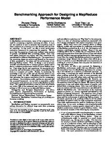
Figure 3: (Top) The flow chart of the proposed EDS approach for mining data streams. (Bottom) The distribution of the eigen values, λmax and λmin with increasing Q for the financial data set, consider here.
Λt,n = diag{λt,i , . . . , λt,j }, be the diagonal matrix with all the noisy eigenvalues. Similarly, let Λt,s = diag{λt,1 , . . . , λt,i−1 , λt,j+1 , . . . , λt,n }, be the diagonal matrix with all the non-random eigenvalues. Let At,n and At,s be the matrices whose columns are eigenvectors corresponding to the eigenvalues in Λt,n and Λt,s , respectively and At = [At,s |At,n ]. Then we can decompose Covt = Covt,s + Covt,n , where 0 Covt,s = At,s Λt,s At,s is the signal part of the covari0 ance matrix and Covt,n = At,n Λt,n At,n is the noise part of the covariance matrix. At any given time step, the signal part of the covariance matrix produces the useful non-random eigenstates and they should be used for data mining applications. Note that it suffices to compute only the eigenvalues (and eigenvectors) that fall outside the interval [λmin , λmax ], corresponding to the signal eigenstates. This allows computation of Covt,s and hence Covt,n . The following section presents the experimental results.
Mobile Financial Data Stream Mining Using EDS
Performance With Respect to Time Random Matrix Based Result 90% Variance Explained Case 75% Variance Explained Case
220 200
2
4
6 8 BATCH NUMBER
10
12
Performance With Respect to Time
ROOT MEAN SQUARE ERROR 3.4 3.6 3.8
Random Matrix Based Result 90% Variance Explained Case 75% Variance Explained Case
3.2
This section describes an application of the EDS for mining Nasdaq 100 financial time-series data streams. The EDS is used to“filter” the correlation matrix for detecting the dependencies among different stocks. The experiments reported here consider 99 companies from Nasdaq 100. We sample data every five minutes and each block of data is comprised of mi = 99 rows. At any given moment the user is interested in the underlying dependencies observed from the current and previously observed data blocks. First let us study the effect of the EDS-based filtering on the eigen-states produced by this financial time-series data. Figure 3(Right) shows the distribution of eigen values from the covariance matrix (Covt ) for different values of t. It also shows the theoretical lower and upper bounds (λmax and λmin ) at different time steps (i.e. increasing Q). The eigen states falling outside these bounds are considered for constructing the “signal” part of the covariance matrix. The figure shows that initially a relatively large number of eigen states are identified as noisy. As time progresses and more data blocks arrive, the noise regime shrinks. It is also interesting to note that the EDS algorithm includes the lower end of the spectrum in the signal part. This is philosophically different from the traditional wisdom of considering only those eigen states with large eigen values. In order to evaluate the online performance of the EDS algorithm we compare the eigen-space captured by the EDS at any given instant with respect to the “true” eigen-space defined by the underlying data distribution. Although data streams are conceptually infinite in size, the experiments documented in this section report results over a finite period of time. So we can benchmark the performance of the EDS with respect to the “true” eigen-space defined by the eigen vectors computed from the entire data set (all the data blocks) collected from the stream during the chosen period of observation. We first report the evolution of the signalpart of the covariance matrix along time and compare that with the “true” covariance matrix generated from the entire data set. We report two different ways to compute this difference:
ERROR 240
260
4
2
4
6 8 BATCH NUMBER
10
12
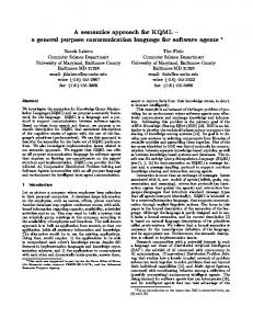
Figure 4: The relative performance (thresholded error count in left and RMS error on right) of the EDS algorithm and the traditional approach using eigen vectors capturing 90% and 75% of the total variance. Different batch numbers correspond to different time steps.
threshold θ then the value is set to 1 otherwise 0. The total number of 1’s in this matrix is the observed thresholded error count. Figure 4 compares the performance of our EDS algorithm with that of a traditional method that simply designates as signal, all the eigen-states that account for, respectively, 90% and 75% of the total variance. It shows the thresholded error count for each method, as a function of time (batch number). It is apparent that the EDS algorithm quickly outperforms the traditional method.
1. RMSE: The root mean square error (RMSE) is computed between the covariance matrices generated by the online EDS and the entire data set.
5
2. Thresholded Error: This measure first computes the difference between the estimated and true covariance matrices. If the (i, j)-th entry of the difference matrix is greater than some user given
This paper described the EDS approach for extracting useful noise-free eigen states from data streams in the context of a mobile data mining application. It showed that the EDS approach is considerably better than the
Conclusions and Future Work
traditional wisdom of selecting the top-ranking eigenvectors guided by some user-given threshold. The EDS allows us to extract the eigenstates that correspond to non-random information that are likely to be useful from a data mining perspective. The EDS approach works by comparing the empirically observed eigen distribution with the known distribution of random matrices. The theoretically known values of upper and lower limits of the spectrum are used to identify the boundary between noisy and signal eigen-states. This random matrix based approach to separating the information bearing and noisy eigenstates has potential computational advantages. Indeed, since the upper bound λmax of the noisy eigenvalues is known a priori, one can easily use a suitable numerical technique (e.g., power method [15]) to compute just the few largest eigenvalues. Once these eigenvalues and corresponding eigenvectors are computed, one can obtain the signal-part of the covariance matrix, which can be subtracted off from the total covariance to isolate the noise-part of the covariance. Another feature of our EDS approach is illustrated in Figure 3. As seen from the graph, the limits λmax and λmin both converge to 1 as the ratio Q tends to infinity (see also equation 1). In a data stream mining scenario, the number of features n is fixed, whereas the number of total number of observations m increases as each block of data is received. Hence, Q increases with time, which results in a smaller interval [λmax , λmin ] for the noisy eigenstates. This means that, as we observe more and more data, the EDS algorithm would potentially designate more eigenstates as signal. This is also intuitively satisfying, since most of the noise would get “averaged-out” as we observe more data.
Acknowledgments The authors acknowledge supports from the United States National Science Foundation CAREER award IIS-0093353 and NASA (NRA) NAS2-37143. The authors would like to thank Li Ding.
References [1] M. L. Mehta. Random Matrices. Academic Press, London, 2 edition, 1991. [2] H. Kargupta, H. Park, S. Pittie, L. Liu, D. Kushraj, and K. Sarkar. Mobimine: Monitoring the stock market from a PDA. ACM SIGKDD Explorations, 3:37–47, 2001. [3] A. Azoff. Neural Network Time Series Forecasting of Financial Markets. Wiley, New York, 1994.
[4] N. Baba and M. Kozaki. An intelligent forecasting system of stock price using neural networks. In Proceedings IJCNN, Baltimore, Maryland, pages 652–657, Los Alamitos, 1992. IEEE Press. [5] S. Cheng. A neural network approach for forecasting and analyzing the price-volume relationship in the taiwan stock market. Master’s thesis, National Jow-Tung University, Taiwan, R.O.C, 1994. [6] R. Kuo, L. Lee, and C. Lee. Intelligent stock market forecasting system through artificial neural networks and fuzzy delphi. In Proceedings of World Congress on Neural Networks, pages 345– 350, San Deigo, 1996. INNS Press. [7] C. Lee. Intelligent stock market forecasting system through artificial neural networks and fuzzy delphi. Master’s thesis, Kaohsiung Polytechnic Institute, Taiwan, R.O.C, 1996. [8] J. Zirilli. Financial Prediction Using Neural Networks. International Thomson Computer Press, 1997. [9] J. Campbell, A. Lo, and A. MacKinley. The Econometrics of Financial Markets. Princeton University Press, USA, 1997. [10] G. Jang, F. Lsi, and T. Parng. Intelligent stock trading decision support system using dual adaptive-structure neural networks. Journal of Information Science Engineering, 9:271–297, 1993. [11] D. Jonsson. Some limit theorems for the eigenvalues of a sample covariance matrix. Journal of Multivariate Analysis, 12:1–38, 1982. [12] H. Hotelling. Analysis of a complex of statistical variables into principal components. Journal of Educational Psychology, 24, 1933. [13] H. Kargupta, K. Sivakumar, and S. Ghosh. Dependency detection in mobimine and random matrices. Accepted for publication in the Proceedings of the 6th European Conference on Principles and Practice of Knowledge Discovery in Databases, 2002. [14] P. Hall, D. Marshall, and R. Martin. Merging and splitting eigenspace models. IEEE Transactions on Pattern Analysis and Machine Intelligence, 22(9):1042–1049, September 2000. [15] J. E. Jackson. A User’s Guide to Principal Components. John Wiley, 1991.