A markov random field approach to spatio ... - Semantic Scholar

2478

IEEE TRANSACTIONS ON GEOSCIENCE AND REMOTE SENSING, VOL. 41, NO. 11, NOVEMBER 2003

A Markov Random Field Approach to Spatio-Temporal Contextual Image Classification Farid Melgani and Sebastiano B. Serpico, Senior Member, IEEE

Abstract—Markov random fields (MRFs) provide a useful and theoretically well-established tool for integrating temporal contextual information into the classification process. In particular, when dealing with a sequence of temporal images, the usual MRF-based approach consists in adopting a “cascade” scheme, i.e., in propagating the temporal information from the current image to the next one of the sequence. The simplicity of the cascade scheme makes it attractive; on the other hand, it does not fully exploit the temporal information available in a sequence of temporal images. In this paper, a “mutual” MRF approach is proposed that aims at improving both the accuracy and the reliability of the classification process by means of a better exploitation of the temporal information. It involves carrying out a bidirectional exchange of the temporal information between the defined single-time MRF models of consecutive images. A difficult issue related to MRFs is the determination of the MRF model parameters that weight the energy terms related to the available information sources. To solve this problem, we propose a simple and fast method based on the concept of “minimum perturbation” and implemented with the pseudoinverse technique for the minimization of the sum of squared errors. Experimental results on a multitemporal dataset made up of two multisensor (Landsat Thematic Mapper and European Remote Sensing 1 synthetic aperture radar) images are reported. The results obtained by the proposed “mutual” approach show a clear improvement in terms of classification accuracy over those yielded by a reference MRF-based classifier. The presented method to automatically estimate the MRF parameters yielded significant results that make it an attractive alternative to the usual trial-and-error search procedure. Index Terms—Artificial neural networks, data fusion, Markov random fields (MRFs), Markov random field (MRF) parameter estimation, multitemporal image classification, spatio-temporal context.

I. INTRODUCTION

T

HE CONTINUOUS enhancement of the satellite remote sensor’s characteristics (e.g., improved spatial and spectral resolutions and reduced revisit time) has increased the importance of remote sensing in real-world applications such as mapping, agriculture, forestry, oil and mineral extraction, fishing, environmental monitoring, and disaster prevention and moni-

Manuscript received October 29, 2002; revised May 9, 2003. This work was supported by the Italian Space Agency (ASI) under research project “Metodi bayesiani basati su Markov Random Fields (MRF) per l’estrazione di informazione da immagini telerilevate.” F. Melgani is with the Department of Information and Communication Technologies, University of Trento, I-38050 Trento, Italy (e-mail: melgani@ dit.unitn.it). S. B. Serpico is with the Department of Biophysical and Electronic Engineering, University of Genoa, I-16145 Genoa, Italy (e-mail: vulcano@ dibe.unige.it). Digital Object Identifier 10.1109/TGRS.2003.817269

toring. In particular, one of the reasons for the growing interest of numerous private and governmental end-users in the exploitation of remote sensing data is represented by the higher quality and larger quantity of information that can be extracted through the analysis of temporal sequences of remote sensing images acquired over a given geographical area. Indeed, focusing on classification-based image analysis, it has been shown in the literature that the integration of the temporal dimension into a classification scheme can significantly improve the results in terms of accuracy and reliability. However, multitemporal-data complexity suggests that a continuous scientific effort is required to develop methodologies capable to better exploit such data and to follow the technological advances of remote sensors. In such a context, Markov random fields (MRFs) [1] represent an effective and theoretically well-established mathematical tool, as they permit one to integrate any contextual information into the classification scheme. In particular, they provide a flexible stochastic framework to model a given scene by expressing spatio-temporal contextual information by means of adequate energy functions. The Hammersley– Clifford theorem [2], which states the Gibbs and Markov random fields equivalence, allows one to reduce the difficulty in defining global distributional models for structured datasets (like images) by considering equivalent models based on local properties of such data. The classification task becomes one of minimizing a total energy function that aggregates the energy functions associated with different information sources. The most widely used algorithms for such a task are the simulated annealing (SA) algorithm, the maximizer of posterior marginals (MPM) algorithm, and the iterated conditional modes (ICM) algorithm [3]. MRFs have proved to be useful not only for classification but also in many other image-processing areas such as image restoration [1], image and texture synthesis [4], [5], segmentation [6]–[8], classification [9], [10], and surface reconstruction [11]. To analyze the temporal context in a sequence of images, the usual approach adopted is the “cascade” approach [12], which represents a natural way to deal with a sequence of temporal images. It consists in propagating the temporal information from the current image to the next one in the sequence. The simplicity of this scheme makes it attractive; however, the “cascade” approach does not fully exploit the temporal information available in a sequence of temporal images. Furthermore, the fact that the information exchange is unidirectional increases the risk of error propagation from a date to the next one. In this paper, a “mutual” approach is proposed that aims at improving both the accuracy and the reliability of the classification

0196-2892/03$17.00 © 2003 IEEE

MELGANI AND SERPICO: MRF APPROACH TO SPATIO-TEMPORAL CONTEXTUAL IMAGE CLASSIFICATION

results by means of a better exploitation of the temporal information. It consists in carrying out a bidirectional exchange of the temporal information between the defined single-time MRF models of consecutive images of a sequence. In the form of an appropriate energy function, each single-time MRF model integrates three basic kinds of information: spectral, spatial contextual, and temporal contextual information. In our approach, we make use of multilayer perceptron (MLP) neural networks to extract spectral information. The use of neural networks is justified by their effective multisensor and multisource fusion capability. Both the spatial and temporal kinds of contextual information are derived from the estimates of the image pixel labels in a given predefined neighborhood system. The estimation of the parameters related to MRF models represents an important issue faced in this paper. Indeed, a critical task when dealing with MRFs is represented by the determination of a good set of the parameters inherent in the MRFs. This is usually accomplished by means of a simple, but above all time-consuming, trial-and-error procedure. Such a problem increases the difficulty in using a powerful mathematical tool like MRFs, thus potentially reducing the interest in it. To overcome this issue, we propose a simple and fast method to automatically estimate the MRF parameters of each MRF model considered in the sequence of temporal images. Experimental results on a multitemporal dataset consisting of two multisensor [Landsat Thematic Mapper (TM) and European Remote Sensing 1 (ERS-1) synthetic aperture radar (SAR)] images are reported and discussed.

II. PREVIOUS WORK Contextual classification has been extensively investigated in the past by the pattern recognition community [13]–[15], in particular, with reference to the spatial context (see [13] for a comprehensive survey). These early works have allowed researchers to establish the basic theoretical frameworks that inspire most of the recent pattern recognition techniques using spatial contextual information. By contrast, research on the use of the temporal context for classification purposes has not been so extensive. Focusing on the classification of remote sensing images, we recall the “cascade” classifier introduced by Swain [12], who generalized the Bayes optimal strategy to the case of multitemporal observations by assuming a class-conditional independence of feature vectors derived from different temporal datasets and by allowing changes in classes over time. The model-based approach proposed by Kalayeh and Landgrebe [16] involves the use of a stochastic system representing land-cover types (through a nonstationary Gaussian process) as input and the temporal spectral behavior as output. The probability of transition from a class at one date to a different class at another date can be used as information to express the correlation of two or more images separate in time. An iterative technique, derived from the Bayes rule for the minimum error, was proposed by Bruzzone and Serpico [17] to estimate the transition probability matrices (TPMs) between classes at two dates. In [18], the TPM is replaced with the joint probability matrix (JPM), computed by applying a specific formulation of the expectation–maximization (E–M) algorithm to a pair of images acquired at different

2479

times. Two techniques, based differently on the concept of the minimum expected cost and dealing with the multitemporal aspect at the decision level, were presented by Jeon and Landgrebe [19]. In [20], a temporal updating approach applied to cloud classification was developed: in order to track temporal changes in a sequence of images, a probabilistic neural network (PNN) classifier is updated on the basis of the maximum-likelihood criterion. Other methods exploit the concept of the temporal signatures of classes; this concept can be expressed, for example, by the Fourier series analysis [21], [22]. However, such methods are constrained by the assumption that no change may occur over time. Finally, only few papers have been published dealing simultaneously with both the spatial and temporal contexts for remote sensing image classification. An interesting (but quite expensive in terms of computation) autocorrelation model was proposed by Khazenie and Crawford [23]: it results from the combination of a class-dependent process with an autocorrelated (spatial and temporal) noise process. MRFs are among the most widely used tools for multitemporal data fusion. Jeon and Landgrebe [24] proposed a cascade spatio-temporal contextual classifier that involves using MRFs to model spatial correlation. MRF capabilities are fully exploited by a general model in [25] to easily merge not only different data sources (including ancillary data) but also spatio-temporal aspects by resorting to simple energy functions. In [26], the change-detection problem is viewed as an inverse ill-posed problem that is solved by using prior knowledge of typical properties of change masks, described as samples from two-dimensional MRFs. In order to increase the accuracy of the final change detection map, Bruzzone and Prieto [27] integrated spatial contextual information in their unsupervised change detection scheme through an MRF model that exploits interpixel class dependences to model the prior probabilities of change and no-change classes. Bruzzone and Prieto [28] also developed an MRF-based adaptive semiparametric technique that makes use of the reduced Parzen estimate (RPE) and the E–M algorithm to estimate in an unsupervised way the changes that may occur in a temporal sequence of images. In [29], the observed temporal images are modeled as MRFs in order to search for an optimal image of changes by applying the maximum a posteriori probability (MAP) decision criterion and the SA energy minimization procedure.

III. METHODOLOGY A. Problem Formulation The proposed mutual approach holds for a general temporal sequence of images. In the following, for the sake of simplicity, we shall focus on an example of sequence of only two temporal images; the extension to several images will be discussed in Section III-C. Let us consider a multitemporal multisensor dataset consisting of two registered images and acquired and at times and , respectively. Let be the sets of possible labels for the related whole scene at times and , respectively. Applying the Bayes rule for the minimum error, the optimal classification of all the pixels of the image acquired at time , given the

2480

IEEE TRANSACTIONS ON GEOSCIENCE AND REMOTE SENSING, VOL. 41, NO. 11, NOVEMBER 2003

image acquired at time and the set of labels for the image , can be performed by applying the MAP decision criterion, i.e., by solving the following maximization problem: Max

(1)

This appears to be a very complicated problem, as it involves the optimization of a global distributional model of the image; hence, it calls for a computationally feasible approximation. By adopting the MRF approach, one can sharply reduce the model complexity by passing from a global model to a model of the local image properties. The latter model is defined in terms of both the potential function of single pixels and the interactions among pixels in appropriate neighborhoods. The combination of the MAP method with the MRF modeling makes the classification task equivalent to the minimization of a total energy expressed in the following relation: function (2) Z where Z is a normalizing constant. The ICM algorithm [30] represents a simple and computationally moderate solution to optimize the MRF–MAP estimates, for it converges to a local, but usually good, minimum of the energy function. In particular, it allows the global optimization problem (2) to be solved by an iterative local optimization. Focusing again on the image , the classification of each pixel of , characterized by the feature vector , is iteratively optimized via the following equation for proportionality [3]: (3) is a possible label to be assigned to the current pixel; where is a set of labels for the image , excluding the current pixel; is a set of labels for the image ; and are suband that corresponds to the labels of the pixels in sets of predefined spatial and temporal neighborhood systems, respecin (3) is unknown, at each tively. As the true set of labels obtained at the previous iteration iteration the estimate of is utilized, according to the ICM algorithm, to generate a new estimate of the label set . Obviously, the set of labels is unknown, too, and needs to be replaced with a proper estimate. In the proposed mutual approach, and are optimized “in parallel,” i.e., at each iteration of the ICM algorithm, the current estimates of and are utilized to generate new estimates of such label sets (see Section III-C). In particular, is optimized by using (a subset of) as temporal context, and is optimized by using (a subset of) as temporal context. We note that, on the contrary, in the cascade approach, the set of labels used in (3) denotes the estimate of the image labels for the image obtained without exploiting the temporal information coming from the image . Such a set remains fixed during the iterations of the ICM estimation procedure applied to classify the image . The minimization of the probability in (3) can be turned again into a problem of energy minimization. In particular, the energy to be minimized for the current pixel takes into account three kinds of information: spectral information, spatial contextual, and temporal contextual information. The separability between spectral information and the two kinds of contextual information is implicit in the ICM algorithm [see (3)]. In addition, for

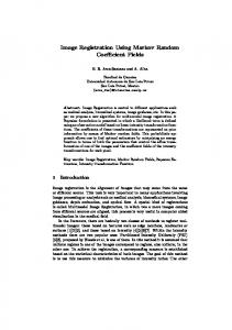
Fig. 1. Spatial (S) and temporal (T) neighborhoods of pixel (p, q) adopted in the case of a temporal sequence of two images.

the sake of simplicity, we assume that also the contributions of the spatial and temporal contexts are separable and additive. Accordingly, the total energy to be minimized for the current pixel becomes (4) , and are the spectral, spatial, and temporal where parameters, respectively. B. Energy Functions 1) Spectral Energy Function: We assume that spectral information can be of the multisensor type. Therefore, in order to fuse multisensor data, we adopt multilayer perceptron (MLP) neural networks, well known for their effective capability to deal with multisource data. Trained by an error back-propagation algorithm to minimize the minimum-square-error (MSE) criterion, they provide the estimates of the single-time posterior probabiland allow us to obtain the noncontextual classifiities cation maps useful to initialize the ICM algorithm. The spectral energy function is then calculated as (5) Other methods to estimate the posterior probabilities can be used as well. 2) Spatial Energy Function: Both the spatial and temporal energy functions require the definition of a neighborhood system. In our case, a second-order neighborhood is adopted, as shown in Fig. 1. The spatial energy function is expressed as (6) where

is the indicator function if otherwise

and is applied to count the number of occurrences of 3) Temporal Energy Function: is defined as

(7) in

. (8)

represents the transition probability from where at time to class at time , i.e., an element of the class so-called TPM. The TPM can be automatically computed (e.g., by using the E–M algorithm [18]). As a simpler alternative, in this paper we propose to compute the TPM by exploiting

MELGANI AND SERPICO: MRF APPROACH TO SPATIO-TEMPORAL CONTEXTUAL IMAGE CLASSIFICATION

Fig. 2.

2481

Block diagram of the proposed mutual spatio-temporal contextual classifier (K is the iteration index).

the expert’s knowledge, represented by allowed transitions and forbidden transitions between classes at different times. Taking into account the prior class probabilities and the appropriate normalization is computed required, the class transition probability as follows: (9)

C. Mutual Approach Up to this point, we have defined the MRF model associated with the image acquired at time ; a similar model can be defined for the image acquired at time . It is worth stressing that in the case of a temporal sequence of two images, the MRF model we adopted for each temporal image is similar to the one proposed in [25], from which it differs in the way the spectral energy is estimated (as will be explained in Section V). A more important difference lies in the manner in which the MRF models are combined. A possible way to deal with a set of multitemporal images is the “cascade” approach adopted in [12] and [25]. For instance, in the case of two images acquired at times and , respectively, the image acquired at time is processed using only spectral and spatial contextual information. Once this image has been processed, the resulting classification map is utilized as temporal information for the image acquired at time . As a consequence, for the classification of the latter image, one can take advantage of temporal information in addition to spectral and spatial information. Obviously, this approach reduces the computational requirements, as compared with the joint (simultaneous) optimization of the classification of both images. However, it does not fully exploit all the available information. The proposed “mutual” approach couples the MRF models (associated with both images) in the energy minimization process carried out by the recursive ICM algorithm (Fig. 2). At each iteration of this algorithm, the previous MRF–MAP estimates for one image are exploited to update the MRF–MAP estimates for

the other image, and vice versa. At convergence, the mutual approach provides a suboptimal solution to the joint classification problem expressed by the following maximization: Max

(10)

where and stand for the labels of the two entire images and , respectively. The optimization algorithm, according to the proposed mutual scheme, can be described as follows. Initialization step: To initialize the ICM procedure, two and are generated with a noninitial label sets contextual classification based on the spectral information only. Toward this end, the MAP criterion is applied to the and posterior probability estimates provided by two MLPs trained with the images acquired at times and , respectively. The values of the param, and are set manually or by a proper eters estimation procedure. th iteration: New estimates and of the label sets and are generated at each iteration, on the basis of and obtained at the previous the estimates iteration, by assigning each pixel of the images and to the class that minimizes the related total energy function. In other words, for every couple of pixels belonging to and , respectively, and corresponding to the images the same location in the images, the following steps are applied: perform the Step 1) For the pixel of the image following: • Compute the single energy func, and tions , and stand for the where sets of spatial and temporal neighboring labels, respectively, derived from the and obtained at estimates the previous iteration.

2482

IEEE TRANSACTIONS ON GEOSCIENCE AND REMOTE SENSING, VOL. 41, NO. 11, NOVEMBER 2003

• Compute the total energy functions , where . • Assign the pixel to the such that label . perform the Step 2) For the pixel of the image following: • Compute the single energy functions , and , with . and are obtained Both and from the previous estimates . It is worth noting that the sets and of spatial contextual labels are identical with the sets of and temporal contextual labels , respectively, without the label of the central pixels. • Compute the total energy functions , where . • Assign the pixel to the such that label Stop criterion: The algorithm is stopped when the numand as compared with bers of different labels in and , respectively, become very small. The extension of the mutual approach to a sequence of more than two images requires that all the images of a given temporal sequence be coupled directly or, at least indirectly, depending on the adopted temporal neighborhood system. For instance, considering a second-order temporal neighborhood system (Fig. 3), a given image takes direct advantage of the temporal informaand of tion coming from the two neighboring images and , in turn, exploit the the sequence. The two images temporal information coming from their respective neighborand , respectively, hood systems, which also include and so on. Accordingly, the image takes indirect advantage of the temporal information propagated also by the images of the temporal sequence that are not covered by the neighborhood system. The optimization algorithm is analogous to that described above, with the difference that it is applied to several images at the same time. In other words, several label sets (i.e., one for each image of the sequence) are initialized at the first iteration; their estimates are then updated at each iteration utilizing the estimates generated at the previous iteration. This scheme, however, may prove unsuitable if all the images of the sequence are not available from the start, but become available progressively. In this case, a simplified scheme may be adopted according to which, instead of running the ICM algorithm on the whole sequence again for each new image, one updates the classification of few images only. For example, if the ICM algorithm has already been applied to a sequence of images and a new image is added later as the last one of the sequence, one can maintain the classification results up to the image and apply again the iterative optimization of the label sets only

Fig. 3. Second-order spatio-temporal neighborhood for a temporal sequence of several images. The neighborhood of the image I is shown.

to the new image and to the previous one only. One ; this system can use the neighborhood system in Fig. 3 for and . For , a reduced includes in its neighborhood both neighborhood system should be adopted that includes only (in a way similar to that used for the image at time in Fig. 1). From a computational viewpoint, in order to evaluate the difference between the proposed mutual approach and the cascade approach, one should consider the number of contextual information sources handled by the two approaches (in addition to the spectral information sources) and the numbers of times and the ways the ICM optimization procedure is applied. In the case of a sequence of two temporal images, the mutual approach requires that the ICM be run only once and that at each iteration, four contextual information sources be updated (two spatial sources and two temporal ones). The cascade approach requires that the ICM be run twice: first, it is applied to the image at time , and only the spatial context is considered; then, it is applied to the image at time , and both the spatial and temporal contexts are considered. Depending on the number of ICM iterations required for convergence, in this case the mutual approach may turn out to be faster. On the contrary, the computational load of the mutual approach increases significantly, compared with that of the cascade approach, in the case where the images of a temporal sequence become progressively available and the mutual approach is applied to each new image to optimize again all the MRF models simultaneously. However, if the above-described simplified scheme is applied whenever a new image is added to the sequence, the number of contextual information sources to be handled by the mutual approach becomes five(one spatial source and two temporal ones for the , and one spatial source and one temporal one for image the image ), whereas for the cascade approach it is equal to 2 (one spatial source and one temporal one). Finally, we note that, if one considers a sequence of images all available from

MELGANI AND SERPICO: MRF APPROACH TO SPATIO-TEMPORAL CONTEXTUAL IMAGE CLASSIFICATION

the start, the ICM is run only once by the mutual approach, contextual information sources, whereas in involving the case of the cascade approach, the ICM needs to be run times, the first time involving only the spatial context, then times involving one spatial context and one temporal one.

2483

the method consists in estimating the values of the three MRF parameters that satisfy the following system of equations:

IV. METHOD FOR MRF PARAMETER ESTIMATION

(14)

MRF models make use of parameters that weigh the influence of information sources on the decision process. This can be viewed as a way of expressing the degree of confidence (reliability) in each information source. In practice, in the context of a supervised classification scheme, the MRF parameters permit one to “tune up” the MRF model in order to optimize classification accuracy. The determination of the MRF parameters is not a trivial problem. The larger the number of information sources, the larger the number of MRF parameters and the more difficult the parameter estimation. It is worth mentioning two automatic methods for MRF parameter estimation, one based on maximum-likelihood estimation [31] and the other one on genetic algorithms [32]. However, both methods appear to be quite demanding in terms of computation. To deal with this issue, in this paper, we propose a simple and fast method for estimating the MRF parameters automatically by means of a “minimum perturbation.” Let us consider for the image at time (the same reasoning holds for the image training samples . at time ) a set of The first step of the method consists in computing for each training sample the total energy associated with each class , under the assumption that all the information sources have the same reliability weights (for convenience, we take them all equal to 1). In other words, the following energy quantity is computed for each sample : (11) , Note that, for the sake of simplicity, we drop the terms in the notation of the energy functions. The optimal and class for the sample is the one that satisfies Min

(12)

We define as “minimal energy perturbation” the smallest additional quantity of energy required to classify the sample correctly (13) stands for the true class of the sample and is where an arbitrary small positive constant. In case the optimal class should correspond to the true class , the minimal energy perturbation would become null. This means that the considered sample does not require any perturbation of its energy function, as it is already correctly classified. Then, after computing the minimal energy perturbation for , the second step of each training sample

where the target

is given by (15)

We aim to find an optimal set of parameters that forces the total energy of the true class to be the minimal one and, consequently, to provide a correct classification of every training sample. A common way to find an approximate solution for such a system characterized by a number of equations larger than the number of unknowns ( equations versus three unknowns) is to adopt the minimization of the sum-of-squared-error as a criterion and to apply the technique based on the pseudoinverse matrix for its optimization. The advantages of the pseudoinverse technique are two: 1) it provides an optimal MSE analytical solution and 2) it is simple and fast. By rewriting the system of (14) in terms of matrices, we obtain (16) is given The estimate of the optimal MRF parameter vector of by the following expression based on the pseudoinverse the matrix : (17) This method is applied in the context of the initialization step of the ICM procedure. For simplicity, the set of estimated paramis then maintained fixed during the iterations of that eters procedure. In any case, if the classification maps do not vary too much from the first iteration to convergence, one can expect that the variations in such parameters through the iterations will be small. Finally, it is worth noting that the proposed MRF parameter estimation method has been developed according to our formulation of the problem of supervised spatio-temporal contextual classification, which handles three sources of information (spectral information and spatial and temporal contextual information). However, it is also applicable to general MRF models involving multiple sources of information (e.g., ancillary data in addition to spatial and temporal contextual information) and, consequently, a larger number of MRF parameters for the supervised classification scheme. V. EXPERIMENTAL RESULTS Located in the basin of the Po river in Northern Italy, the considered scene is an agricultural area shown in two registered temporal images acquired by the Landsat TM and ERS-1 SAR sensors in April and May 1994, respectively (Fig. 4). At each date, eleven features were extracted, i.e., six intensity features from the Landsat TM image, one intensity feature from

2484

IEEE TRANSACTIONS ON GEOSCIENCE AND REMOTE SENSING, VOL. 41, NO. 11, NOVEMBER 2003

(a)

(b)

Fig. 4. Multisensor images acquired over a part of the basin of the Po river (Northern Italy), in May 1994 by (a) Landsat TM (band 5) and (b) ERS-1 SAR (C-band, VV polarization).

the ERS-1 SAR (C-band, VV polarization) image, and four texture features (entropy, difference entropy, correlation, and sum variance) extracted from the ERS-1 SAR image by computing the gray-level cooccurrence matrix [33]. The main land covers in the April image were four: wet areas, bare soil, cereals fields, and woods. In the May image, the typology of the land-cover classes changed a little to span five information classes: dry and wet areas, cereals and corn fields, and woods. Two training sets were necessary: the first (TRAIN1) was used to train the neural networks, whereas the MRF parameters were estimated on the basis of the second training set (TRAIN2). In addition, an independent test set (TEST) was considered to assess the accuracies of the different classifiers. The numbers of training and test pixels used in the experiments are given in Table I for each class and each date. The prior probabilities and ] were estimated by using the of the classes [ training sets. The two transition probability matrices (TPMs) were computed on the basis of the information provided by experts (Table II). In order to assess the performances of the different classifiers, two accuracy measures are utilized in the following: the “Overall Accuracy” (OA), which is the percentage of correctly classified pixels among all the pixels considered (independently of the classes they belong to) and the “Average Accuracy” (AA), which is the average over the classification accuracies obtained for the different classes. For each date, a two-layer perceptron neural network (MLP), with 11 input nodes, ten hidden nodes, and a number of output nodes corresponding to the number of classes (four for April

TABLE I NUMBERS

OF

TRAINING

AND TEST PIXELS FOR (a) THE AND (b) THE MAY IMAGE

APRIL IMAGE

(a)

(b)

and five for May), was trained using the back-propagation algorithm. The two MLPs made it possible to produce the initial classification map for each date, in addition to the single-time posterior probabilities required by the MRF-based spatio-temporal contextual classifiers. Table III(a) and (b) provides the results of the MLP classifiers on the test samples of the April and May images, respectively, in terms of OA, AA, and single-class accuracies (see the first row of each table). Even though the results were obtained without using any spatio-temporal contextual information, they are rather good. The main problem is

MELGANI AND SERPICO: MRF APPROACH TO SPATIO-TEMPORAL CONTEXTUAL IMAGE CLASSIFICATION

TABLE II CLASS TPMs. (a) FROM APRIL TO MAY. (b) FROM MAY (“CER” STANDS FOR “CEREALS”)

TO

APRIL

(a)

(b)

the discrimination of the class “cereals” in April, with an accuracy of just 26.8%. This can be explained by two reasons: 1) the fact that the class “cereals” is in the minority and 2) the overlap of this class (in the spectral distribution) with the background-cover class, i.e., the class “bare soil.” However, as this plant grows in the April–May period, the image taken in May allowed a better accuracy to be obtained (68.9%). For the purpose of comparison, an MRF-based classifier similar to that described in [25] was implemented, with the only difference that instead of the multivariate normal class-conditional probability density function, the sensor-specific class-conditional energy function (spectral energy function) is expressed by means of the class posterior probabilities provided by the MLPs [as expressed in (5)]. The two possible “cascade” schemes (from April to May and from May to April) were implemented in order that the results on both images might take advantage of temporal contextual information. A good set of MRF parameters was found empirically by fixing and exploring different combinations of and , first with a rough step (0.5), then with a fine step (0.05) around the best combination previously found. The following values were , and (for the “April obtained: , and to May” scheme) and (for the “May to April” scheme). Six iterations were necessary for the two cascade MRF-based classifiers (CMRFs) to reach convergence and yield their final results. The computation time required by each cascade scheme to classify both the first and second images was approximately equal to 90 min on a personal computer with a 1.2-GHz processor. The mutual MRF-based classifier (MMRF) achieved convergence also at the sixth iteration by using the empirical parameter values , and for the MRF models of both the first and second images. In this case, the computation time spent to classify both images was about 50 min with the same machine. The results obtained by the CMRF and MMRF classifiers are shown in Table III in terms of classification accuracy. The integration of spatio-temporal contextual information showed its benefits in the sharp improvement in accuracy for the class “cereals”; some significant improvements were also obtained by the “cascade” and “mutual” approaches for the

2485

TABLE III OVERALL ACCURACY (OA), AVERAGE ACCURACY (AA), AND SINGLE-CLASS ACCURACIES (EXPRESSED IN PERCENT) OBTAINED BY THE NONCONTEXTUAL (MLP) AND CONTEXTUAL (CMRF, MMRF, and MMRF ) CLASSIFIERS ON (a) THE SET OF TEST SAMPLES OF THE APRIL IMAGE AND (b) THE SET OF TEST SAMPLES OF THE MAY IMAGE

(a)

(b)

other classes at both dates (April and May). Comparing the two approaches, the proposed MMRF classifier proved to be more effective, with a 15.5% increase in the AA (against 10.8% obtained by the CMRF one) for the April image. This is mainly explained by the gain in accuracy for the class “cereals” in April (60.6% by the MMRF classifier against 41.6% by the CMRF one). For the May image, the MMRF classifier turned out to be more accurate than the CMRF one, with a gain of 2.2% against 0.6% in the OA, and a gain of 4.7% against a loss of 1.3% in the AA. The CMRF showed a decrease in accuracy for the class “cereals” 4.7% against a 20.0% gain by the MMRF. The decrease in accuracy for the class “cereals” is explained by the fact that in the “April-to-May” cascade scheme, the temporal information deriving from the same class in the April image represented a misleading information source because of the poor accuracy obtained for that class (26.8%). As the CMRF classifier is based on a unidirectional exchange of temporal information, it involved a propagation of error from the April image to the May image; the error propagation mainly concerned the class “cereals.” The implementation of the proposed automatic method for MRF parameter optimization allowed us to obtain results (indicated with MMRF in Table III) that were, for both MRF models, very similar to those yielded by the trial-and-error procedure and, in some cases, slightly better (Table III). As expected from our theoretical formulation of the MRF-parameter estimation problem, this confirms that the proposed method permits one to obtain, in an automatic way, a good solution in the space of “classification accuracy versus parameter values.” In other words, it allows an effective tuning of the parameters of each MRF model that determine the relative importance of the spectral, spatial contextual, and temporal contextual information. The two sets of parameter values found in few seconds by using the second training set (TRAIN2) were and for the MRF models associated with the April and May images, respectively. In order to assess the stability of the MRF tuning parameters to the evolution of the contextual information during the iterations of the ICM procedure, we computed again such a set of parameters after con-

2486

IEEE TRANSACTIONS ON GEOSCIENCE AND REMOTE SENSING, VOL. 41, NO. 11, NOVEMBER 2003

vergence, and found the following values: for the April image and for the May image. These results confirm that the values of the above parameters are quite stable, at least in the cases like the present one, i.e., when the classification maps do not vary too much during the iterations of the ICM procedure.

VI. CONCLUSION The results reported in this paper show that the integration of spatio-temporal contextual information into the classification scheme considerably improves the accuracy values over those obtained by using a conventional noncontextual classification method. Markov random fields provide a flexible and powerful theoretical framework to model a multitemporal scene for the purpose of classification. The flexibility of such a tool results from its ability to aggregate multitype information (including ancillary data [25]) into the same model; its simplicity also depends on the way the energy functions are defined. In our case, we adopted a relatively simple neighborhood system of the second order; nonetheless, the adopted model yielded interesting results. In a multitemporal context, the way in which the MRF models are combined plays a key role in the classification scheme. A better exploitation of spatio-temporal contextual information allowed the proposed “mutual” approach to provide better results than the usual “cascade” approach, thus proving to be an interesting and valid alternative to it. In particular, the mutual approach reduces the risk of propagating the classification error from one image at one date to another image at another date, as confirmed in the experiments by the accuracy of the class “cereals” in May. An appropriate setting of the transition probability matrices (TPMs) is important, as the related values may in general affect the accuracy of classification results. An automatic approach (such as the algorithm based on expectation maximization [18]) appears to be the best choice, specially when a sequence of many images is to be processed. However, in this paper, we have shown that the proposed method allows one to improve classification results also in the case where the TPMs are derived in a simple way, i.e., just indicating allowed and forbidden transitions on the basis of the expert’s knowledge. For each temporal image, a preprocessing step is required to estimate the parameters of the corresponding MRF model. Indeed, the parameters may vary from one model to another, as each model captures the characteristics intrinsic to the related image. The preprocessing step is usually based on a trial-anderror procedure for parameter setting; therefore, it may turn out to be tricky and time consuming. The proposed method for the automatic MRF parameter estimation represents an attractive and computationally feasible solution to the problem. Indeed, only few seconds were necessary to automatically estimate a set of parameters that provided results very similar to (in some case, slightly better than) those obtained by a set of parameters empirically found after a several-hour trial-and-error search.

Even though the proposed method for parameter estimation is fast, quite a long computation time is required to extract contextual information and to include it in the classification process by the MRF approach. However, we note that this is not the most time-consuming task of the overall processing and classification chain we adopted. In particular, the overall computation time required to classify the two images was equal to several hours, which included the time to compute the texture features from the SAR images, the time required to train the two neural networks, and the time to apply these networks to the entire images (for noncontextual classification and spectral information extraction). Processing could be made faster by improving the code of the software modules utilized, which were developed in our lab and were not optimized from the viewpoint of computation speed. ACKNOWLEDGMENT The authors wish to thank M. A. Gomarasca [Consiglio Nazionale delle Ricerche y Istituto per il Rilevamento Elettromagnetico dell’Ambiente (CNR-IREA)] for providing the multitemporal images used in the experiments and the related ground truth. Support by the Italian Space Agency for this work is gratefully acknowledged. REFERENCES [1] S. Geman and D. Geman, “Stochastic relaxation, Gibbs distributions, and the Bayesian restoration of images,” IEEE Trans. Pattern Anal. Machine Intell., vol. PAMI-6, pp. 721–741, 1984. [2] J. Besag, “Spatial interaction and the statistical analysis of lattice systems (with discussion),” J. R. Statist. Soc. B, vol. 36, pp. 192–326, 1974. [3] R. C. Dubes and A. K. Jain, “Random field models in image analysis,” J. Appl. Statist., vol. 16, pp. 131–163, 1989. [4] R. Chellappa and R. L. Kashyap, “Texture synthesis using spatial interaction models,” IEEE Trans. Acoust., Speech Signal Processing, vol. ASSP-33, pp. 194–203, Feb. 1985. [5] G. R. Cross and A. K. Jain, “Markov random field texture models,” IEEE Trans. Pattern Anal. Machine Intell., vol. PAMI-5, pp. 25–39, Jan. 1983. [6] H. Derin, H. Elliott, R. Cristi, and D. Geman, “Bayes smoothing algorithms for segmentation of binary images modeled by Markov random fields,” IEEE Trans. Pattern Anal. Machine Intell., vol. PAMI-6, pp. 707–720, 1984. [7] S. Krishnamachari and R. Chellappa, “Multiresolution Gauss–Markov random field models for texture segmentation,” IEEE Trans. Image Processing, vol. 6, pp. 251–267, Feb. 1997. [8] S. A. Barker and P. J. W. Rayner, “Unsupervised image segmentation using Markov random field models,” Pattern Recognit., vol. 33, pp. 587–602, 2000. [9] H. Derin and H. Elliott, “Modeling and segmentation of noisy and textured images using Gibbs random fields,” IEEE Trans. Pattern Anal. Machine Intell., vol. PAMI-9, pp. 39–55, Jan. 1987. [10] Z. Kato, J. Zerubia, and M. Berthod, “Unsupervised parallel image classification using Markovian models,” Pattern Recognit., vol. 32, pp. 591–604, 1999. [11] D. Geiger and F. Girosi, “Parallel and deterministic algorithms from MRFs: Surface reconstruction,” IEEE Trans. Pattern Anal. Machine Intell., vol. 13, pp. 401–412, May 1991. [12] P. H. Swain, “Bayesian classification in a time-varying environment,” IEEE Trans. Syst., Man, Cybern., vol. SMC-8, pp. 879–883, 1978. [13] J. Kittler and J. Föglein, “Contextual classification of multispectral pixel data,” Image Vis. Comput., vol. 2, pp. 13–29, 1984. [14] G. T. Toussaint, “The use of context in pattern recognition,” Pattern Recognit., vol. 10, pp. 189–204, 1978. [15] R. M. Haralick, “Decision making in context,” IEEE Trans. Pattern Anal. Machine Intell., vol. PAMI-5, pp. 417–428, 1983. [16] H. M. Kalayeh and D. A. Landgrebe, “Utilizing multitemporal data by a stochastic model,” IEEE Trans. Geosci. Remote Sensing, vol. 24, pp. 792–795, 1986.

MELGANI AND SERPICO: MRF APPROACH TO SPATIO-TEMPORAL CONTEXTUAL IMAGE CLASSIFICATION

[17] L. Bruzzone and S. B. Serpico, “An iterative technique for the detection of land-cover transitions in multitemporal remote-sensing images,” IEEE Trans. Geosci. Remote Sensing, vol. 35, pp. 858–867, July 1997. [18] L. Bruzzone, D. F. Prieto, and S. B. Serpico, “A neural-statistical approach to multitemporal and multisource remote-sensing image classification,” IEEE Trans. Geosci. Remote Sensing, vol. 37, pp. 1350–1359, May 1999. [19] B. Jeon and D. A. Landgrebe, “Decision fusion approach for multitemporal classification,” IEEE Trans. Geosci. Remote Sensing, vol. 37, pp. 1227–1233, May 1999. [20] B. Tian, M. R. Azimi-Sadjadi, T. H. Vonder Haar, and D. Reinke, “Temporal updating scheme for probabilistic neural network with application to satellite cloud classification,” IEEE Trans. Neural Networks, vol. 11, pp. 903–920, July 2000. [21] L. Olsson and L. Eklundh, “Fourier series for analysis of temporal sequences of satellite sensor imagery,” Int. J. Remote Sens., vol. 15, pp. 3735–3741, 1994. [22] L. Andres, W. A. Salas, and D. Skole, “Fourier analysis of multi-temporal AVHRR data applied to a land cover classification,” Int. J. Remote Sens., vol. 15, pp. 1115–1121, 1994. [23] N. Khazenie and M. M. Crawford, “Spatio-temporal autocorrelated model for contextual classification,” IEEE Trans. Geosci. Remote Sensing, vol. 28, pp. 529–539, July 1990. [24] B. Jeon and D. A. Landgrebe, “Classification with spatio-temporal interpixel class dependency contexts,” IEEE Trans. Geosci. Remote Sensing, vol. 30, pp. 663–672, July 1992. [25] A. H. S. Solberg, T. Taxt, and A. K. Jain, “A Markov random field model for classification of multisource satellite imagery,” IEEE Trans. Geosci. Remote Sensing, vol. 43, pp. 100–113, Jan. 1996. [26] T. Aach and A. Kaup, “Bayesian algorithms for adaptive change detection in image sequences using Markov random fields,” Signal Process.: Image Commun., vol. 7, pp. 147–160, 1995. [27] L. Bruzzone and D. F. Prieto, “Automatic analysis of the difference image for unsupervised change detection,” IEEE Trans. Geosci. Remote Sensing, vol. 38, pp. 1171–1182, May 2000. , “An adaptive semiparametric and context-based approach to un[28] supervised change detection in multitemporal remote-sensing images,” IEEE Trans. Image Processing, vol. 11, pp. 452–466, Apr. 2002. [29] T. Kasetkasem and P. K. Varshney, “An image change detection algorithm based on Markov random field models,” IEEE Trans. Geosci. Remote Sensing, vol. 40, pp. 1815–1823, Aug. 2002. [30] J. Besag, “On the statistical analysis of dirty pictures,” J. R. Statist. Soc. B, vol. 48, pp. 259–302, 1986. [31] X. Descombes, R. D. Morris, J. Zerubia, and M. Berthod, “Estimation of Markov random field prior parameters using Markov chain Monte Carlo maximum likelihood,” IEEE Trans. Image Processing, vol. 8, pp. 954–963, July 1999. [32] B. C. K. Tso and P. M. Mather, “Classification of multisource remote sensing imagery using a genetic algorithm and Markov random fields,” IEEE Trans. Geosci. Remote Sensing, vol. 37, pp. 1255–1260, May 1999. [33] R. M. Haralick, K. Shanmugam, and I. Dinstein, “Textural features for image classification,” IEEE Trans. Syst., Man, Cybern., vol. SMC-3, pp. 610–621, 1973.

2487

Farid Melgani received the State Engineer degree in electronics from the University of Batna, Batna, Algeria, in 1994, the M.Sc. degree in electrical engineering from the University of Baghdad, Baghdad, Iraq, in 1999, and the Ph.D. degree in electronic and computer engineering from the University of Genoa, Genoa, Italy, in 2003. From 1999 to 2002, he cooperated with the Signal Processing and Telecommunications Group, Department of Biophysical and Electronic Engineering, University of Genoa. He is currently an Assistant Professor in telecommunications at the University of Trento, Trento, Italy, where he teaches pattern recognition, radar remote sensing systems, and digital transmission. His research interests are in the area of processing and pattern recognition techniques applied to remote sensing images (classification, multitemporal analysis, and data fusion). He is coauthor of more than 20 scientific publications. Dr. Melgani served on the Scientific Committee of the SPIE International Conferences on Signal and Image Processing for Remote Sensing VI (Barcelona, Spain, 2000) and VII (Toulouse, France, 2001) and is a referee for the IEEE TRANSACTIONS ON GEOSCIENCE AND REMOTE SENSING.

Sebastiano B. Serpico (M’87–SM’00) received the laurea degree in electronic engineering and the Ph.D. degree in telecommunications from the University of Genoa, Genoa, Italy, in 1982 and 1989, respectively. Since 1982, he has cooperated with the Department of Biophysical and Electronic Engineering (DIBE), University of Genoa, in the field of image processing and recognition. As an Assistant Professor with DIBE, from 1990 to 1998, he has taught pattern recognition, signal theory, telecommunication systems, and electrical communication. Since 1998, he has been an Associate Professor of telecommunications at the Faculty of Engineering, University of Genoa, where he currently teaches signal theory and pattern recognition. His current research interests include the application of pattern recognition (feature selection, classification, change detection, and data fusion) to remotely sensed images. From 1995 to the end of 1998, he was Head of the Signal Processing and Telecommunications Research Group (SP&T) at DIBE and is currently Head of the SP&T Laboratory. He is the author or coauthor of more than 150 scientific publications, including journals and conference proceedings. Dr. Serpico was the recipient of the Recognition of TGARS Best Reviewers from the IEEE Geoscience and Remote Sensing Society in 1998 and was a Guest Editor (with Professor D. A. Landgrebe) of a Special Issue of the IEEE TRANSACTIONS ON GEOSCIENCE AND REMOTE SENSING on the subject of the analysis of hyperspectral image data (July 2001). Since 2001, he has been an Associate Editor of the TRANSACTIONS ON GEOSCIENCE AND REMOTE SENSING. He is a member of the International Association for Pattern Recognition Society (IAPR).