Oct 23, 2017 - and the tensor train [2] format made quite an impact, as both formats al- ... lation of the tensor train SVD (TT-SVD) for general higher order ...
arXiv:1710.08513v1 [math.NA] 23 Oct 2017
A Randomized Tensor Train Singular Value Decomposition Benjamin Huber, Reinhold Schneider and Sebastian Wolf 25th October 2017 Abstract The hierarchical SVD provides a quasi-best low rank approximation of high dimensional data in the hierarchical Tucker framework. Similar to the SVD for matrices, it provides a fundamental but expensive tool for tensor computations. In the present work we examine generalizations of randomized matrix decomposition methods to higher order tensors in the framework of the hierarchical tensors representation. In particular we present and analyze a randomized algorithm for the calculation of the hierarchical SVD (HSVD) for the tensor train (TT) format.
1
Introduction
Low rank matrix decompositions, such as the singular value decomposition (SVD) and the QR decomposition are principal tools in data analysis and scientific computing. For matrices with small rank both decompositions offer a tremendous reduction in computational complexity and can expose the underlying problem structure. In recent years generalizations of these low rank decompositions to higher order tensors have proven to be very useful and efficient techniques as well. In particular the hierarchical Tucker [1] and the tensor train [2] format made quite an impact, as both formats allow to circumvent the notorious curse of dimensionality, i.e. the exponential scaling of the ambient spaces with respect to the order of the tensors. Applications of these formats are as various as high-dimensional PDE’s like the Fokker Planck equations and the many particle Schr¨odinger equations, applications in neuroscience, graph analysis, signal processing, computer vision and computational finance, see the extensive survey of Grasedyck et
1
al. [3]. Also in a recent paper in machine learning Cohen et al. [4] showed a connection between these tensor formats and deep neural networks and used this to explain the much higher power of expressiveness of deep neural networks over shallow ones. One of the main challenges when working with these formats is the calculation of low rank decompositions of implicitly or explicitly given tensors, i.e. the high dimension analog of the classical SVD calculation. For matrices there exists a wide range of methods, which allow these calculations with high efficiently and precision. One particular branch are randomized methods which appear often in the literature, mostly as efficient heuristics to calculate approximate decompositions. It was only recently that thanks to new results form random matrix theory, a rigorous analysis of these procedures became possible, see [5]. In this work we aim to extend some of these results for randomized matrix decompositions to the high dimensional tensor case. To this end we present an algorithm which allows the efficient calculation of the tensor train SVD (TT-SVD) for general higher order tensors. Especially for sparse tensors this algorithms exhibits a superior complexity, scaling only linear in the order, compared to the exponential scaling of the naive approach. Extending the results of [5], we show that stochastic error bounds can also be obtained for these higher order methods. This work focuses on the theoretical and algorithmic aspects of this randomized (TT-)SVD. However a particular application on our mind is the work in [6, 7], where we treat the tensor completion problem. That is, in analogy to matrix completion, see e.g. [8–10], we want to reconstruct a tensor from N measurements using a low rank assumption. We use an iterative (hard) thresholding procedure, which requires the (approximate) calculation of a low rank decomposition in each iteration of the algorithm. As the deterministic TT-SVD is already a fundamental tool, there are of course many further possible application for our randomized variant, see for example [11–13]. We start with a brief recap of tensor product spaces and introduce the notation used in the remainder of this work. In section 2 we give an overview of different tensor decompositions, generalizing the singular value decomposition from matrices to higher order tensors. In the second part a detailed introduction of the tensor train format is provided. Section 3.1 summarizes results for randomized matrix decompositions which are important for this work. In section 3.2 we introduce our randomized TT-SVD scheme
2
and prove stochastic error bounds for this procedure. An interesting relation between the proposed algorithm and the popular alternating least squares (ALS) algorithm is examined in section 4. Section 5 collects several numerical experiments showing the performance of the proposed algorithms. Section 6 closes with some concluding remarks.
1.1
Tensor product spaces
Let us begin with some preliminaries on tensors and tensor spaces. For an exhaustive introduction we refer to the monograph of Hackbusch [14]. Given Hilbert spaces V1 , . . . ,Vd the tensor product space of order d V =
d O
Vi ,
i=1
is defined as the closure of the span of all elementary tensor products of vectors from Vi , i.e. V := span {v1 ⊗ v2 ⊗ . . . ⊗ vd | vi ∈ Vi } . The elements x ∈ V are called tensors of order d. If each space Vi is supplied with an orthonormal basis {ϕµi i : µi ∈ N}, then any x ∈ V can be represented as ∞ ∞ x=
∑
µ1 =1
...
∑
x[µ1 , . . . , µd ] ϕµ11 ⊗ · · · ⊗ ϕµdd .
µd =1
Using this basis, with a slight abuse of notation, we can identify x ∈ V with its representation by a d-variate function, often called hyper matrix, µ = (µ1 , . . . , µd ) 7→ x[µ1 , . . . , µd ] ∈ K , depending on discrete variables, usually called indices µi ∈ N. Analogous to vectors and matrices we use square brackets x[µ1 , . . . , µd ] to index the entries of this hypermatrix. Of course, the actual representation of x ∈ V depends on the chosen bases ϕ i of Vi . The index µi is said to correspond to the µ-th mode or equivalently the µ-th dimension of the tensor. In the remainder of this article, we confine to finite dimensional real linear spaces Vi := Rni , however most parts are easy to extend to the complex case as well. For these, the tensor product space V =
d O
Rni = Rn1 ×n2 ×...×nd := span {v1 ⊗ v2 ⊗ . . . ⊗ vd | vi ∈ Rni }
i=1
3
is easily defined. If it is not stated explicitly, the Vi = Rni are supplied with the canonical basis {ei1 , . . . , eini } of the vector spaces Rni . Then every x ∈ V can be represented as nd
n1
x=
∑
...
µ1 =1
∑
x[µ1 , . . . , µd ] e1µ1 ⊗ · · · ⊗ edµd .
(1)
µd =1
We equip the finite dimensional linear space V with the inner product nd
n1
hx, yi :=
∑
µ1 =1
···
∑
x[µ1 , . . . , µd ] y[µ1 , . . . , µd ] .
µd =1
p and the corresponding l2 -norm kxk = hx, xi. We use the fact that for a Hilbert space Vi the dual space V ∗ is isomorphic to Vi and use the identification V ' V ∗ . For the treatment of reflexive Banach spaces we refer to [15, 16]. The number of possibly non-zero entries in the representation of x is n1 · · · nd = Πdi=1 ni , and with n = max{ni : i = 1, . . . , d}, the dimension of the space V scales exponentially in d, i.e. O(nd ). This is often referred to as the curse of dimensions and presents the main challenge when working with higher order tensors.
1.2
Tensor Contractions and Diagrammatic Notation
Important concepts for the definitions of tensor decompositions are so called matricizations and contractions introduced in this section. The matricization or flattening of a tensor is the reinterpretation of the given tensor as a matrix, by combining a subset of modes to a single mode and combining the remaining modes to a second one. Definition 1 (Matricization or Flattening). Let [n] = {1, 2, . . . , n} and x ∈ Rn1 ×...×nd be a tensor of order d. Furthermore let α ⊆ [d] be a subset of the modes of x, and let β = [d]\α be its complement. Given two bijective functions µα : [nα1 ] × [nα2 ] × . . . → [nα1 · nα2 · · · ] and µβ respectively. The α-matricization or α-flattening Mˆ α : Rn1 ×...×nd → Rmα ×mβ x 7→ Mˆ α (x)
4
of x is defined entry-wise as � � x[i1 , . . . , id ] =: Mˆ α (x) µα (iα1 , iα2 . . .), µβ (iβ1 , iβ2 , . . .) . A common choice for µα and µβ is µ(i1 , i2 , . . .) = ∑k ik ∏ j>k n j . The actual choice is of no significance though, as long as it stays consistent. The matrix dimensions are given as mα = ∏ j∈α n j and mβ = ∏ j∈β n j . The inverse operation is the de-matricization or unflattening Mˆ −1 . In principle it is possible to define de-matricization for any kind of matrix, typically called tensorization. However this requires to give the dimensions of the resulting tensor and the details of the mapping alongside with the operator. Instead, in this work the de-matricization is only applied to matrices where at least one mode of the matrix encodes a tensor structure through a former matricization, in which the details of the mapping are clear from the context. For all other modes the de-matricization is simply defined to be the identity. The second important tool are tensor contractions, which are generalizations of the matrix-vector and matrix-matrix multiplications to higher order tensors. Definition 2 (Tensor Contraction). Let x ∈ Rn1 ×...×nd and y ∈ Rm1 ×...×me be two tensors of order d and e respectively, with nk = ml . The contraction of the k-th mode of u with the l-th mode of v z := x ◦k,l y is defined entry-wise as z[i1 , . . . , ik−1 , ik+1 , . . . , id , j1 , . . . , jl−1 , jl+1 , . . . , je ] nk
=
∑ x[i1 , . . . , ik−1 , p, ik+1 , . . . , id ] y[ j1 , . . . , jl−1 , p, jl+1 , . . . , je ]
p=0
or via the matricizations � z = Mˆ −1 Mˆ {k} (x)T Mˆ {l} (y) . The resulting tensor z ∈ Rn1 ×...×nk−1 ×nk+1 ×...×nd ×m1 ×...mk−1 ×mk+1 ×...×me is of order d + e − 2. Note that in order for this operation to be well-defined, nk = ml must hold.
5
If no indices are specified, i.e. only ◦, a contraction of the last mode of the left operand and the first mode of the right operand is assumed. If tuples of indices are given, e.g. ◦(i, j,k),(l,p,q) , a contraction of the respective mode pairs (i/l, j/p k/q) is assumed.1 As writing this for larger tensor expressions quickly becomes cumbersome we also use a diagrammatic notation to visualize the contraction. In this notation a tensor is depicted as a dot or box with edges corresponding to each of its modes. If appropriate the cardinality of the corresponding index set is given as well. From left to right the following shows this for an order one tensor (vector) v ∈ Rn , an order two tensor (matrix) A ∈ Rm×n and an order 4 tensor x ∈ Rn1 ×n2 ×n3 ×n4 . n3 n
v
A
m
n4 x
n
n1 n2
If a contraction is performed between the modes of two tensors the corresponding edges are joined. The following shows this exemplary for the inner product of two vectors u, v ∈ Rn and a matrix-vector product with A ∈ Rm×n and v ∈ Rn . u
n
v
m
A
n
v
There are two special cases concerning orthogonal and diagonal matrices. If a specific matricization of a tensor yields an orthogonal or diagonal matrix, the tensor is depicted by a half filled circle (orthogonal) or a circle with a diagonal bar (diagonal) respectively. The half filling and the diagonal bar both divide the circle in two halves. The edges joined to either half, correspond to the mode sets of the matricization, which yields the orthogonal or diagonal matrix. As an example the diagrammatic notation can be used to depict the singular value decomposition A = USVT of a matrix A ∈ Rm×n with rank r, as shown in the following. U
r
S
m
1 As
r
V n
one can easily show the order of the contractions does not matter.
6
2
Low Rank Tensor Decompositions
In this section we give an introduction to the low rank tensor decomposition techniques used in the remainder of this work. As there are in fact quite different approaches to generalize the singular value decomposition, and thereby also the definition of the rank, to higher order tensors, we start with an overview of the most popular formats. For an in depth overview including application we refer to the survey of Grasedyck et al. [3]. In the second part we provide a detailed introduction of the tensor train format, which is used in the remainder of this work. The probably best known and classical tensor decomposition is the representation by a sum of elementary tensor products, i.e. r
x = ∑ u1,i ⊗ u2,i ⊗ . . . ⊗ ud,i
(2)
i=1
where x ∈ Rn1 ×...×nd and uk,i ∈ Rnk are vectors from the respective vector spaces. This format is mainly know as the canonical format but also appears in the literature under the names canonical polyadic (CP) format, CANDECOMP and PARAFAC. The canonical or CP rank is defined as the minimal r such that a decomposition as in (2) exists. Note that in general there is no unique CP representation with minimal rank. This is somewhat expected, since even for matrices the SVD is not unique if two or more singular values coincide. Some discussion on the uniqueness can be found in the paper of Kolda and Bader [17]. For tensors with small canonical rank (2) offers a very efficient representation, requiring only O(rdn) storage instead of O(nd ) for the direct representation. Unfortunately the canonical format suffers from several difficulties and instabilities. First of all the task of determining the canonical rank of a tensor with order d > 2 is, in contrast to matrices, highly non trivial. In fact it was shown by [18] that even for order d = 3, the problem of deciding whether a rational tensor has CP-rank r is NP-hard (and NP-complete for finite fields). Consequently also the problem of calculating low rank approximations proves to be challenging. That is, given a tensor x ∈ Rn1 ×...×nd and a CP-rank r, finding the best CP-rank r approximation x∗ =
argmin
(kx − yk) .
(3)
y∈Rn1 ×...×nd , CP-rank(y)≤r
The norm k·k used, may differ depending on the application. In the matrix case the Eckart-Young theorem provides that for the Frobenius and spectral norm this best approximation can be straightforwardly calculated by a
7
truncated SVD. In contrast, De Silva and Lim [19] proved that the problem of the best CP-rank r approximation, as formulated in (3), is ill-posed for many ranks r ≥ 2 and all orders d > 2 regardless of the choice of the norm k·k. Furthermore they showed that the set of tensors that do not have a best CP-rank r approximation is a non-null set, i.e. there is a strictly positive probability that a randomly chosen tensor does not admit a best CP-rank r approximation. Finally it was shown by De Silva and Lim [19] that neither the set {x ∈ Rn1 ×...×nd | CP-rank(x) = r} of all tensors with CP-rank r, nor the set {x ∈ Rn1 ×...×nd | CP-rank(x) ≤ r} of all tensors with CP-rank at most r is closed for d > 2. These are some severe difficulties for both the theoretical and practical work with the canonical format. The second classical approach to generalize the SVD to higher order tensors is the subspace based Tucker decomposition. It was first introduced by Tucker [20] in 1963 and has been refined later on in many works, see e.g. [14, 17, 21]. Given a tensor x ∈ Rn1 ×...×nd , the main idea is to find minimal subspaces Ui ⊆ Rni , such that x ∈ Rn1 ×...×nd is an element of the induced tensor space U =
d O
Ui ⊆
i=1
d O
Rni = Rn1 ×...×nd .
i=1
� Let ri = dim(Ui ) denote the dimension of the i-th subspace and let ui, j , j = 0, . . . , ri be an orthonormal basis of Ui . If the subspaces are chosen such that x ∈ U , then (1) states that there is a c such that x can be expressed as rd
r1
x=
∑
ν1 =1
. . . ∑ c[ν1 , ν2 , . . . , νd ] · u1,ν1 ⊗ . . . ⊗ ud,νd . νd
Usually the basis vectors are combined to orthogonal matrices Ui = (ui,1 , . . . , ui,ri ), called basis matrices. This leads to the following common form of the Tucker format r1
x[µ1 , . . . , µd ] =
∑
ν1 =1
rd
. . . ∑ c[ν1 , . . . , νd ]U1 [µ1 , ν1 ] . . . Ud [µd , νd ] .
(4)
νd
The order d tensor c ∈ Rr1 ×...×rd of the prefactors is usually called core tensor. The d-tuple r = (r1 , r2 , . . . , rd ) of the subspace dimensions is called the representation rank and is associated with the particular representation. The Tucker rank (T-rank) of x is defined as the unique minimal d-tuple r∗ = (r1∗ , . . . , rd∗ ), such that there exists a Tucker representation of x with rank
8
n6
n5 n5
n6
r5 n1
n4
n4
r6 r1
r4
n3 n2
r3
n1
r2
n3
n2
Figure 1: Left: A tensor x ∈ Rn1 ×...×n6 of order 6. Right: Its Tucker decomposition. r∗ . Equation (4) consists of d tensor contractions, that can be visualized in the diagrammatic notation, which is exemplarily shown in Figure 1 for d = 6. Note that even for the minimal T-rank, the Tucker decomposition is not unique, as for any orthogonal matrix Qi ∈ Rri ×ri , one can define a matrix ˜ i = Ui Qi and the tensor U ri
c˜ [µ1 , . . . , µd ] =
∑ c [µ1 , . . . , ν, . . . µd ] QT [ν, µi ] ν=1
such that the tensor x can also be written as rd
r1
u [µ1 , . . . , µd ] =
∑
ν1 =1
...
∑ c˜ [ν1 , . . . , νd ] U1 [µ1 , ν1 ] . . . U˜ i [µi , νi ] . . . Ud [µd , νd ],
vd =1
which is a valid Tucker decomposition with the same rank. It is shown by De Lathauwer et al. [21] that the Tucker rank as the minimal d-tuple is indeed well-defined and that the entries ri of the Tucker rank correspond to the rank of the i-th mode matricization of the tensor. That is � T-rank(x) = rank(Mˆ {1} (x)), . . . , rank(Mˆ {d} (x)) . The proof is tightly linked to the fact, that a Tucker representation of a tensor x ∈ Rn1 ×...×nd with minimal representation rank, can be obtained by successive singular value decompositions. This procedure is referred to as the higher order singular value decomposition (HOSVD), see [21] for the details. Using truncated SVDs an approximation of x by a tensor x∗ with lower T-rank r∗ = (r1∗ , . . . rd∗ ) � (r1 , . . . , rd ), can be obtained. Where the symbol �
9
denotes an entry-wise ≤, i.e. (r1 , . . . rd ) � (r1∗ , . . . , rd∗ ) ⇐⇒ ri ≤ ri∗ ∀i. In contrast to the Eckart-Young theorem for matrices the approximation x∗ ob∗ approximation of x. However it tained in this way is not the best T-rank r√ is a quasi-best approximation by a factor d, i.e. √ kx − x∗ kF ≤ d min (kx − ykF ) . y : T-rank(y)�r∗
For many applications this quasi-best approximation is sufficient. As for the canonical format, finding the true best approximation is at the very least NPhard in general, as it is shown by [22] that finding the best rank (1, . . . , 1) approximation is already NP-hard. To store a tensor in the Tucker format only the core tensor and the basis matrices have to be stored. This amounts to a storage requirement of O(rd + dnr), where r := max(r1 , . . . , rd ) and n := max(n1 , . . . , nd ). Compared to the O(nd ) this is a major reduction but does not break the curse of dimensionality as the exponential scaling in d remains. A more recent development is the hierarchical Tucker (HT) format, introduced by Hackbusch and K¨uhn [1]. It inherits most of the advantages of the Tucker format, in particular a generalized higher order SVD, see [23]. But in contrast to the Tucker format the HT format allows a linear scaling with respect to the order for the storage requirements and common operations for tensors of fixed rank. The main idea of the HT format is to extend the subspace approach of the Tucker format by a multi-layer hierarchy of subspaces. For an in-depth introduction of the hierarchical Tucker format we refer to the pertinent literature, e.g. [1, 14, 23]. In this work we will instead focus on the tensor train (TT) format, as introduced by Oseledets [2]. The TT format offers mostly the same advantages as the more general HT format, while maintaining a powerful simplicity. In fact it can to some extend be seen as a special case of the HT format, see Grasedyck and Hackbusch [24] for details on the relation between the TT and HT format.
2.1
Tensor Train Format
In this subsection we give a detailed introduction to the tensor train (TT) format. In the formulation used in this work the TT format was introduced by Oseledets [2], however an equivalent formulation was known in quantum physic for quite some time, see e.g. [25] for an overview. The idea of the TT-format is to separate the modes of a tensor into d order two and three tensors. This results in a tensor network that is exemplary shown for an order four tensor x = W1 ◦ W2 ◦ W3 ◦ W4 in the following diagram.
10
W1 r1 n1
W3
W2 r2 n2
W4 r3
n3
n4
Formally it can be defined as follows. Definition 3 (Tensor Train Format). Let x ∈ Rn1 ×...×nd be a tensor of order d. A factorization x = W1 ◦ W2 ◦ . . . ◦ Wd−1 ◦ Wd ,
(5)
of x, into component tensors W1 ∈ Rn1 ×r1 , Wi ∈ Rri−1 ×ni ×ri (i = 2, . . . , d − 1) and Wd ∈ Rrd−1 ×nd , is called a tensor train (TT) representation of x. Equivalently (5) can be given entry-wise as x[i1 , . . . , id ] =
∑ . . . ∑ W1 [i1 , j1 ] W2 [ j1 , i2 , j2 ] . . . Wd−1 [ jd−2 , id−1 , jd−1 ] Wd [ jd−1 , id ] . j1
jd−1
The tuple of the dimensions r = (r1 , . . . , rd−1 ) of the component tensors is called the representation rank and is associated with the specific representation. In contrast the tensor train rank (TT-rank) of x is defined as the min∗ ) such that there exists a TT representation imal rank tuple r∗ = (r1∗ , . . . , rd−1 of x with representation rank equal to r∗ . As for the Tucker format the TT-rank is well defined and linked to the rank of specific matricizations via � TT-Rank(x) = rank(Mˆ {1} (x)), rank(Mˆ {1,2} (x)), . . . , rank(Mˆ {1,2,...,d−1} (x)) . The proof is again closely linked to the fact that a tensor train decomposition of an arbitrary tensor can be calculated using successive singular value decompositions. This procedure is commonly referred to as the TT-SVD. For this work the TT-SVD is of particular importance as it constitutes the deterministic baseline for our randomized approach in section 3.2. In the following we therefore provide a complete step by step description of this procedure. Tensor Train Singular Value Decomposition (TT-SVD) The intuition of the TT-SVD is that in every step a (matrix) SVD is performed to detach one open mode from the tensor. Figure 2 shows this process step by step for an order four tensor and is frequently referred to in
11
the following description. The TT-SVD starts by calculating an SVD of the matricization of x = x0 , where all modes but the first one are combined (Fig. 2 (a)-(c)) � U1 S1 VT1 := SVD Mˆ {1} (x0 ) , with U1 ∈ Rn1 ×r1 , S1 ∈ Rr1 ×r1 , VT1 ∈ Rr1 ×(n2 ·...·nd ) . The dimension r1 is equal � T ˆ to the rank of M{1} (x0 ). The resulting matrices S1 V1 and U1 are each dematricized, which is trivial for U1 in the first step (Fig. 2 (d)-(e)). W1 := Mˆ −1 (U1 ) � x1 := Mˆ −1 S1 VT1
W1 ∈ Rn1 ×r1 x1 ∈ Rr1 ×n2 ×...×nd
Note that there holds � W1 ◦ x1 = Mˆ −1 U1 S1 VT1 = x0 = x . In the next step a matricization of the newly acquired tensor x1 is performed. The first dimension of the matricization is formed by the first two modes of x1 , corresponding to the new dimension introduced by the prior SVD and the second original dimension. The second dimension of the matricization is formed by all remaining modes of x1 (Fig. 2 (f)). From this matricization another SVD is calculated (Fig. 2 (g)) � U2 S2 VT2 := SVD Mˆ {1,2} (x1 ) , (r1 ·n2 )×r2 , S ∈ Rr2 ×r2 , VT ∈ Rr2 ×(n3 ·...·nd ) . As in the first step U with U2 ∈ R 2 2 2 � T and S2 V2 are then dematricized (Fig. 2 (i)),
W2 := Mˆ −1 (U2 ) x2 := Mˆ −1 (S2 VT2 )
W2 ∈ Rr1 ×n2 ×r2 x2 ∈ Rr2 ×n3 ×...×nd
and again there holds � W2 ◦ x2 = Mˆ −1 U2 S2 VT2 = x1 ⇒ W1 ◦ W2 ◦ x2 = x . The obtained rank r2 is equal to the rank of the matricization Mˆ {1,2} (x), which can be shown as follows. First note that Q := Mˆ {1,2} (U1 ◦ U2 ) ∈
12
n2
Mˆ (1) (x0 )
x0
n1
n3
n1
U1
S1
n2 n3 n4
r1
n4
r1
n1
(a)
n2 n3 n4
(b)
W1 Mˆ (1) (x1 )
(c)
n2
W1
r1 n2 n3 n4
n3
(d)
r1
n4
n1
Mˆ (1,2) (x1 )
W1
x1
r1
n1
V1
r1 n2
n1
(e)
W1
U2
S2
r1 n2
r1
r2
V2
(f) Mˆ (1,2) (W2 ) Mˆ (1) (x2 )
W1
r2
n1
r1 n2
r1 n3 n4
n3 n4 (h)
W2
x2
r1
r2
n1
r2
n1
(g) W1
n3 n4
W1 n4
n2
r1
n3
Mˆ (1,2) (x2 )
W2 r2
n1
r2 n3
n4
n2 (j)
(i) W1
Mˆ (1,2) (W3 ) S2
W2 r1
n1
r2
r2 n3
r3
V2 r3
n2
n4 (k)
W1 r1 n1
Mˆ (1,2) (W3 ) U4
W2 r2
r2 n3
n2
W1
r3
W3
W2 r1
n4
n1
(l)
r2 n2
W4 r3
n3
n4
(m)
Figure 2: Step by step depiction of the TT-SVD by example for an order 4 tensor. 13
R(n1 ·n2 )×r2 is an orthogonal matrix, because � QQT [ j, j0 ] = ∑ Mˆ {1,2} (W1 ◦ W2 ) [i, j] Mˆ (1,2) (W1 ◦ W2 ) [i, j0 ] i
=
i1 ,i2
=
W1 [i1 , k] W2 [k, i2 , j] W1 [i1 , k0 ] W2 [k0 , i2 , j0 ]
∑
,k,k0
∑ ∑ W1 [i1 , k] W1 [i1 , k0 ] W2 [k, i2 , j] W2 [k0 , i2 , j0 ]
i2 ,k,k0 i1
|
{z
I[k,k0 ]
}
= ∑ W2 [k, i2 , j] W2 [k, i2 , j0 ] i2 ,k
= I[ j, j0 ] . Then consider that Mˆ {1,2} (x) = Mˆ {1,2} (W1 ◦ W2 ◦ x3 ) = Mˆ {1,2} (W1 ◦ W2 ) Mˆ {1} (x2 ) = QS2 VT2 holds. This is a valid SVD of Mˆ {1,2} (x) and since the matrix of singular values is unique it follows that in fact rank(Mˆ {1,2} (x)) = r2 . This procedure is continued for a total of d − 2 steps and in each step the order of xi ∈ Rri ×ni+1 ×...×nd shrinks by one. Furthermore there holds
Wi ∈ Rri−1 ×ni ×ri step (Fig. 2 (k))
W1 ◦ W2 ◦ . . . ◦ Wi ◦ xi = x � and ri = rank Mˆ {1,...,i} (x) in every step. The (d − 1)-st � Ud−1 Sd−1 VTd−1 = SVD Mˆ {1,2} (xd−1 ) ,
with Ud−1 ∈ R(rd−2 ·nd−1 )×rd−1 , Sd−1 ∈ Rrd−1 ×rd−1 , VTd−1 ∈ Rrd−1 ×nd , is special since the de-matricization of (Sd−1 VTd−1 ), yields an order two tensor that is named Wd instead of xd (Fig. 2 (l)-(m)) Wd−1 = Mˆ −1 (Ud−1 )
Wd−1 ∈ Rrd−2 ×nd−1 ×rd−1 xd ∈ Rrd−1 ×nd .
Wd = Sd−1 VTd−1 Finally
W1 ◦ W2 ◦ . . . ◦ Wd−1 ◦ Wd = x
14
is a valid TT representation of x with TT-rank r = (r1 , . . . , rd−1 ), whose entries ri = rank(Mˆ {1,...,i} (x)) are exactly the ranks of the matricizations as asserted. ∗ ) The same algorithm can also be used to calculate a rank r∗ = (r1∗ , . . . , rd−1 approximation of a tensor x ∈ Rn1 ×...×nd with TT-rank r � r∗ . To this end the normal SVDs are replaced by truncated rank ri∗ SVDs, yielding a tensor x∗ of TT-rank r∗ . In contrast to the matrix case, x∗ is in general not the best rank r∗ approximation of x. However as shown by [2], it is a quasi best approximation with √ kx − x∗ k2 ≤ d − 1 min (kx − yk) . y : TT-rank(y)�r∗
The computational complexity of the TT-SVD is dominated by the d − 1 matrix singular value decompositions, with all other contributions being asymptotically negligible. With n := max(n1 , . . . , nd ) and r := max(r1 , . . . rd ) 2 d−i ) ⊂ O(dnd+1 ), i.e. still exponential the cost scales as O(nd+1 + ∑d−1 i=1 r n in the order. This is somewhat expected because there are in general nd entries in the original tensor that have to be considered. Unfortunately x being sparse or otherwise structured incurs no dramatic change because the structure is generally lost after the first SVD. Apart from the generalized singular value decomposition the TT format offers several further beneficial properties. In particular it is able to break the curse of dimensionality, in the sense that the storage complexity of a tensor x ∈ Rn1 ×...×nd with TT-rank r = (r1 , . . . , rd−1 ) in a minimal TT representation scales as O(dnr2 ), i.e. linearly in the order. Here n := maxi (n1 , . . . , nd ) and r := maxi (r1 , . . . , rd−1 ). Additionally also the computational complexity of common operations as additions and scalar products, scale only linearly in the order for fixed ranks, see [2, 14]. Another desirable property is that the set of tensors with rank at most r form a closed set and as shown by Holtz et al. [26] the set of tensor with exact rank r forms a smooth manifold, allowing the application of Riemannian optimization techniques [27, 28] and dynamical low rank approximation [29, 30], see also the review article [12]. Especially for numerical applications these properties made the tensor train one of, if not the, most popular tensor decomposition of recent years.
15
3
Randomized SVD for higher order tensors
As shown in the previous section calculating a low rank representation or approximation of a given higher order tensor is a challenging task, as the complexity of the tensor train SVD (TT-SVD) scales exponentially in the order. For dense tensors this is of course somewhat expected as there is an exponential number of entries that have to be incorporated. Nevertheless also for sparse and structured matrices the two decomposition techniques exhibit an exponential scaling. In this section we look at randomized methods for the calculation of approximate matrix factorizations. For sparse or structured matrices these techniques allow for a very efficient calculation of common matrix factorizations such as the SVD or QR decomposition, while offering rigorous stochastic error bounds. In the second part of this section we apply these results to formulate randomized TT-SVD algorithms. We show that there hold stochastic error bounds similar to the matrix setting. We also show that this randomized TT-SVD has only linear complexity with respect to the order when applied to sparse tensors.
3.1
Randomized SVD for matrices
Randomized techniques for the calculation of SVD or QR factorizations of matrices have been proposed many times in the literature. However it was only recently that, thanks to the application of new results from random matrix theory these procedures could be analyzed rigorously. We start this section by presenting some results from the work of Halko et al. [5], which will provide a solid basis for the randomized tensor factorization methods of the second part of this section. In this part we restrict ourself to standard Gaussian random matrices, i.e. matrices whose entries are i.i.d. standard Gaussian random variables. The usage of structured random matrices is discussed in section 6. In the formulation of Halko et al. [5], the basis of all decompositions is a randomized method to calculate an approximate low rank subspace projection A ≈ QQT A
(6)
where A ∈ Rn×m is a given matrix and Q ∈ Rn×s is an orthogonal matrix approximately spanning the range of A. Here s = r + p, where r is the desired rank and p is an oversampling parameter. With this projection at hand
16
numerous different low rank decompositions can be calculated deterministically at low costs. For example the singular value decomposition of A can be calculated by forming B := QT A and calculating the deterministic SVD ˜ = QU USVT = B of B. Using U ˜ T = QQT A ≈ A USV is an approximate SVD of A containing only the approximation error incurred by the subspace-projection. The computational costs of the involved � operations scale as O sTmult + s2 (m + n) , where Tmult is the cost to calculate the matrix-vector product with A, which is O(mn) for a general matrix but can be much lower for structured or sparse matrices. In a similar way other matrix factorizations can also be computed with low costs if the projection (6) is given. The main challenge is the calculation of the approximate range Q through random techniques. For this [5] present the following prototype algorithm. Given a matrix A ∈ Rn1 ×n2 .
Listing 1: Randomized range approximation I n p u t : A, r, p O u t p u t : Q C r e a t e a s t a n d a r d G a u s s i a n random m a t r i x G ∈ Rn2 ×(r+p) C a l c u l a t e t h e i n t e r m e d i a t e m a t r i x B := AG ∈ Rn1 ×s . Compute t h e f a c t o r i z a t i o n QR = B . The following theorem proves that the Q obtained in this manner is indeed an approximation of the range of A in the sense of (6). Theorem 1 (Halko et al. [5]). Given A ∈ Rm×n and s = r + p with p ≥ 2. For the projection Q obtained by procedure 1 there holds the following error bounds. h i p kA − QQT Ak ≤ 1 + 11 (r + p) · min(m, n) σr+1 with probability at least 1 − 6p−p and for p ≥ 4 and any u,t ≥ 1 " T
kA − QQ Ak ≤ 1 + t
s
12r p
!1/2
#
∑
σk2
k>r 2 /2
with probability at least 1 − 5t −p − 2e−u
17
.
√ e r+ p σr+1 + ut p+1
Let us highlight furthermore that for the operator norm, we have that σr+1 = inf rank B=r kA − Bkop and for the Frobenius norm there holds ! 21
∑ σk2 k>r
3.2
=
inf
kA − Bk .
rank(B)≤r
Randomized TT-SVD
In this section we show how the same idea of the randomized range approximation for matrices can be used to formulate a randomized algorithm that calculates an approximate TT-SVD of arbitrary tensors. We show that stochastic error bounds analogous to the matrix case can be obtained. Furthermore we show that for sparse tensors this randomized TT-SVD can be calculated in linear complexity with respect to the order of the tensor, instead of the exponential complexity of the deterministic TT-SVD. The idea of our randomized TT-SVD procedure is to calculate nested range approximations increasing by one mode at a time. The corresponding projector is composed of separated orthogonal parts, which are calculated using procedure 1. This is visualized in figure 3. These orthogonal parts will become the component tensors W2 , . . . , Wd of the final TT decomposition. The first component tensor W1 is given by contracting the initial x with all orthogonal components, i.e. W1 = x ◦(2,...,d),(2,...,d) (W2 ◦ . . . ◦ Wd ) The exact procedure calculating the orthogonal components and this final contraction is given in listing 2.
Listing 2: Randomized TT-SVD I n p u t : x , O u t p u t : W1 , . . . , Wd S e t bd+1 := x F o r j = d, . . . , 2 : C r e a t e a G a u s s i a n random t e n s o r g ∈ Rs j−1 ×n1 ×...×n j−1 C a l c u l a t e a j := g ◦(2,... j),(1,..., j−1) b j+1 C a l c u l a t e t h e f a c t o r i z a t i o n R j Q j := Mˆ {1} (a j ) S e t W j := Mˆ −1 (Q j ) if j = d: C a l c u l a t e b j = b j+1 ◦( j),(2) W j
18
Bd x
x ≈
Qd = Wd Qd = Wd
bd
bd
x
x ≈
Wd−1 Wd−1
bd−1
bd−1
x
x ≈
Wd−2 Wd−2
.. . Figure 3: Iterative construction of the tensor bi by subsequent range approximations.
19
B2 x
x = Pˆ2,...,d
Figure 4: Depiction of the randomized TT-SVD as the action of the projection operator Pˆ2,...,d else C a l c u l a t e b j = b j+1 ◦( j, j+1),(2,3) W j S e t W1 = b2 At the end of the procedure in listing 2 x ≈ W1 ◦ W2 ◦ W3 ◦ . . . ◦ Wd is an approximate TT decomposition of rank s = (s1 , . . . , sd−1 ). This final composition can also be given in terms of contractions with the orthogonal parts, i.e. x ≈ W1 ◦ W2 ◦ W3 ◦ . . . ◦ Wd � = x ◦(2,...,d),(2,...,d) (W2 ◦ . . . ◦ Wd ) ◦ W2 ◦ W3 ◦ . . . ◦ Wd = x ◦(2,...,d),(2,...,d) ((W2 ◦ . . . ◦ Wd ) ◦1,1 (W2 ◦ . . . ◦ Wd )) =: Pˆ2,...,d (x) where the effect of the orthogonal parts can also be seen as the action of an projector Pˆ2,...,d . Note that since all parts are orthogonal this is indeed an orthogonal projector. This relation is visualized in figure 4. In the following it will be useful to also define the orthogonal projections Pˆi,...,d (x) := x ◦(i,...,d),(i,...,d) ((Wi ◦ . . . ◦ Wd ) ◦1,1 (Wi ◦ . . . ◦ Wd )) . The following theorem shows that there exists an stochastic error bound for this randomized TT-SVD. Theorem 2 (Error bound). Given x ∈ Rn1 ×...×nd , s = r + p with p ≥ 4. For every u,t ≥ 1 the error of the randomized TT-SVD, as given in listing 2,
20
fulfills kx − P2..d (x)k ≤
√ d − 1 η(r, p)
min
kx − yk
(7)
TT-rank(y)≤r
2
with probability at least (1 − 5t −p − 2e−u /2 )d−1 . The parameter η is given as s √ 12r e r+ p η = 1+t + ut . p p+1 �T Proof. For syntactical convenience let use define Bi := Mˆ {1,...,i−1} (bi ) . Then as Pˆ2,...,d is an orthogonal projector we have kx − P2..d (x)k2 = kxk2 − kP2..d (x)k2
� = kxk2 − B2 , B2
� = kxk2 − Q2 B3 , Q2 B3
� = kxk2 − B3 , QT2 Q2 B3 .
(8)
For all 2 ≤ i ≤ d there holds
�
� Bi+1 , QTi Qi Bi+1 = Bi+1 , Bi+1 − (I − QTi Qi )Bi+1
� = kBi+1 k2 − Bi+1 , (I − QTi Qi )Bi+1 = kBi+1 k2 − k(I − QTi Qi )Bi+1 k2
� = Bi+2 , QTi+1 Qi+1 Bi+2 − k(I − QTi Qi )Bi+1 k2 , where we used that QTi Qi is an orthogonal projector as well. Inserting this iteratively into (8) gives d
kx − P2..d (x)k2 = kxk2 − kBd+1 k2 + ∑ k(I − QTi Qi )Bi+1 k2 i=2
d
= ∑ k(I − QTi Qi )Bi+1 k2 , i=2
where we used that Bd+1 as a matricization of bd+1 := x has the same norm as x itself. As Qi is obtained in the exact setting of theorem 1, we know that
21
for all i k(I − Qi QTi )Bi+1 k2 2 s ! !1/2 √ 12r e r+ p σr+1 (Bi+1 ) ≤ 1+t σk2 (Bi+1 ) + ut ∑ p p + 1 k>r s ! !1/2 2 √ e 12r r + p ≤ 1+t + ut ∑ σk2 (Bi+1 ) p p+1 k>r ≤ η 2 ∑ σk2 (Bi+1 ) k>r 2
holds with probability at least 1 − 5t −p − 2e−u /2 . Note that the singular values of Bi+1 are the same as of Mˆ {1,...,i−1} (Pˆi+1..d (x)), see e.g. figure 4. As shown by Hochstenbach and Reichel [31] the application of an orthogonal projection can only decrease the singular values. Thereby it follows that k(I − Qi QTi )Bi+1 k2 ≤ η 2 ∑ σk2 (Bi+1 ) k>r
=η
2
≤η
2
≤η
2
∑ σk2 (Mˆ {1,...,i−1} (Pˆi+1..d (x))) k>r
∑ σk2 (Mˆ {1,...,i−1} (x)) k>r
≤ η2
min
rank(Mˆ {1,...,i−1} (y))≤r
min
kx − yk2
kx − yk2 .
TT-rank(y)≤r
As the random tensors g are sampled independently in each step, the combined probability that the above holds for all i is at least ρ ≥ (1 − 5t −p − 2 2e−u /2 )d−1 , as asserted. Note that if the tensor x actually has TT-rank r or smaller, that is if minTT-rank(y)≤r kx−yk = 0, then the randomized TT-SVD is exact with probability one. This follows directly from theorem 2 by using t → ∞, u → ∞. Using standard Gaussian random tensors the computational complexity of the randomized TT-SVD is bounded by O(dsnd ), which is very similar to the deterministic TT-SVD presented in section 2.1. However, as we show in the following proposition 1, for sparse tensors the complexity scales only linearly in the order, which is a dramatic reduction compared to the exponential scaling of the deterministic TT-SVD.
22
Proposition 1. Assume that x ∈ Rn1 ×...×nd contains at most N non-zero entries. Then the computational complexity of the randomized TT-SVD given in listing 2 scales as O(d(s2 N + s3 n)). Proof. First note that if x has at most N non-zero entries then each bi has at most si−1 N non-zero entries. The fact that x has at most N non-zero entries implies that, independent of j, there are at most N tuples (k1 , . . . , k j ) such that the sub-tensor x[k1 , . . . , k j , ·, . . . , ·] is not completely zero. Now each bi can be given as bi = x ◦(i,...,d),(2,...,d−i+1) (Wi ◦ . . . ◦ Wd ). As any contraction involving a zero tensors results in a zero tensor, bi is non zero only if the first d − i + 1 modes take values according to the at most N tuples. As there is only one further mode of dimension si−1 there can in in total be only si−1 N non-zero entries in bi . Creating only the, at most s j−1 s j N, entries of g actually needed to perform the product a j := g ◦(2,... j),(1,..., j−1) b j+1 this calculation can be done in O(s j−1 s j N). Calculating the QR of Mˆ (1) (a j ) has complexity O(s2j−1 n j s j ). The involved (de-)matrification actually do not incur any computational costs. Finally the product b j = b j+1 ◦( j, j+1),(2,3) Wd− j has complexity O(s j−1 s j N). These steps have to be repeated d − 1 times. Adding it all up this gives an asymptotic cost bounded by O(d(s2 N + s3 n)), where s := max(s1 , . . . , sd ).
4 Relation to the Alternating Least Squares (ALS) Algorithm There is an interesting connection between the proposed randomized TTSVD and the popular alternating least squares (ALS) algorithm, which is examined in this section. Most of this section is still work in progress but we consider sharing the ideas worthwhile nevertheless. The ALS itself is a general optimization algorithm, highly related to the very successful DMRG algorithm known in quantum physics. We provide only a minimal introduction and refer to the literature for an exhaustive treatment, see e.g. [32, 33]. The ALS is used to solve optimization problems on the set of tensors with fixed TT-rank r, for general objective functionals J : Rn1 ×...×nd → R. The special case interesting in this work is J (x) := kf − xk2
23
for a given tensor f ∈ Rn1 ×...×nd . The global optimum is then exactly the best rank r approximation x∗ := argminTT-rank(y)=r ky − fk . Observing that the parametrization x = τ (W1 , . . . , Wd ) = W1 ◦ . . . ◦ Wd is multi-linear in the parameters Wi ∈ Rri−1 ×ni ×ri . Hence fixing all components W1 except the i-th component Ui , provides a parametrization of x which is linear in Ui ∈ Rri−1 ×ni ×ri , x := x(Ui ) := W1 ◦ . . . ◦ Ui ◦ . . . ◦ Wd Therefore the original optimization problem in the large ambient space Rn1 ×...×nd is restricted or projected onto a relatively small subspace Rri−1 ×ni ×ri , where it can be easily solved, � Wi := argminUi ∈Rri−1 ×ni ×ri kW1 ◦ . . . ◦ Ui ◦ . . . ◦ Wd − fk2 . This procedure is then continued iteratively by choosing another component W j to be optimized next, resulting in a nonlinear Gauß Seidel iteration. The process of optimizing each component exactly once is often called a halfsweep. Although these ideas can also be applied for the canonical format and general tensor networks as well, the tensor train and hierarchical Tucker format admit the possibility to use an orthonormal bases, which can be directly derived from the components Wi by corresponding (left/right) orthogonalization. With this simple post processing step, the ALS algorithm performs much better and more stable than without orthogonalization see eg. [32]. To get started, the ALS algorithm requires an initial guess, i.eit needs d − 1 (left /right) orthogonal components. A usual choice is to use (Gaussian) random tensors for the d − 1 components, possibly orthogonalized. The interesting observation is that using these random initialization one half-sweep can almost be cast to our proposed randomized TT-SVD and vice versa, in the sense that numerically exactly the same operations are performed. The only difference is that, in the picture of the randomized TT-SVD, the random tensor g is not chosen as a Gaussian random tensor in each step but as the first d − i (contracted) random components of the ALS initialization. Note that this means that for the matrix case d = 2 the two methods actually coincide completely. Would it be possible to extend our error bounds to the setting of using structured random tensors g and also to cope with the stochastic dependence implied by the fact that g of different
24
steps are not sampled independently, one could for example prove stochastic error bounds for the first sweep of the ALS. Possible not only for the low rank approximation setting but also for more general objective functionals J . Numerical results indeed do suggest that such extensions might be possible. However this is devoted to forthcoming research.
5
Numerical Experiments
In order to provide practical proof of the performance of the presented randomized TT-SVD we conducted several numerical experiments. All calculations were performed using the xerus C++ toolbox [34], which also contains our implementation of the randomized TT-SVD. The random tensors used in the following experiments are created as follows. Standard Gaussian random tensors are created by sampling each entry independently from N (0, 1). Sparse random tensors are created by sampling N entries independently from N (0, 1) and placing them at positions sampled independently and evenly distributed from [n1 ] × [n2 ] × . . . × [nd ]. The low rank tensors are created by sampling the entries of the component tensors W1 , . . . , Wd in representation (5), independently from N (0, 1), i.e. all components Wi are independent standard Gaussian random tensors. In some experiments we impose a certain decay for the singular values of the involved matrifications. To this end we create a all random components as above, then for i from 1 to d − 1 we contract Wi ◦ Wi+1 and then re-separate them by calculating the SVD USVT , but replacing the S with a matrix S˜ in which the singular values decay in the desired way. For a quadratical decay that is 1 S˜ := diag(1, 212 , 312 , . . . , 250 2 , 0, . . . , 0), where 250 is a cut-off used in all experiments below. Then set Wi = Mˆ −1 (U) and Wi+1 = Mˆ −1 (SVT ). Note that since the later steps change the singular values of the earlier matrification, the singular values of the resulting tensor do not obey the desired decay exactly. However empirically we observed that this method yields a sufficiently well approximation for most applications, even after a single sweep. A general problem is that, as described in section 2.1 the calculation of the actual best rank r approximation of higher order tensors is NP-hard in general. Moreover to the authors knowledge there are no non-trivial higher order tensors for which this best approximation is known in advance. Therefore a direct check of our stochastic error bound (7) using the actual best approximation error is unfeasible. Instead most of the numerical experiments use the error of the deterministic TT-SVD introduced in section 2.1 for com-
25
Relative errors εrnd and εdet
0.25
Randomized TT-SVD samples Randomized TT-SVD average Classical TT-SVD samples Classical TT-SVD average
0.2 0.15 0.1 0.05 0 0.1
0.08
0.06 0.04 Noise level τ
0.02
0
Figure 5: Approximation error of deterministic and randomized TT-SVD in dependency to the noise level. Parameters are d = 10, n = 4, r∗ = 10, r = 10, p = 5. √ parison, which gives a quasi best approximation. The factor of d − 1 is present in both error bounds, but the remaining error dependence given by (7) is verifiable in this way. If not stated otherwise we use the same values for all dimensions ni = n, target ranks ri = r and (approximate) ranks of the solution ri∗ = r∗ . In derogation from this rule the ranks are always chosen within the limits of the dimensions of the corresponding matrifications. For example for d = 8, n = 4, r = 20 the actual TT-rank would be r = (4, 16, 20, 20, 20, 16, 4). 256 samples are calculated for each point, unless specified otherwise. The results for the randomized TT-SVD are obtained by calculating an rank r + p approximation as described in section 3.2 and then use the deterministic TT-SDV to truncate this to rank r. This is done so that in all experiments the randomized and the deterministic approximation have identical final ranks r.
5.1
Approximation Quality for Nearly Low Rank Tensors
In this experiment we examine the approximation quality of the randomized TT-SVD for almost exact low rank tensors. I.e. we create random
26
TT-rank r∗ tensors xexact ∈ Rn×...×n and standard Gaussian random tensors n ∈ Rn1 ×...×nd . The target tensor is then created as x :=
n xexact +τ , kxexact k knk
for some noise level τ. Subsequently rank r approximations ydet and yrnd of x are calculate using the randomized and deterministic TT-SVD. Finally we examine the relative errors εdet :=
kx − ydet k kxk
εrnd :=
kx − yrnd k . kxk
Figure 5 show these errors for different noise levels τ. The parameters are chosen as d = 10, n = 4, r∗ = 10, r = 10, p = 5, with 256 samples calculated for each method and noise level. As expected the error of the classical TT-SVD almost equals the noise τ for all samples, with nearly no variance. Independent of the noise level, the error εrnd of the randomized TT-SVD is larger by a factor of approximately 1.6. The only exception is in the case τ = 0 where both methods are exact up to numerical precision. In contrast to the classical TT-SVD, there is some variance in the error εrnd . Notably this variance continuously decreases to zero with the noise level τ. These observations are in agreement with the theoretical expectations, as theorem 2 states that the approximation error of the randomized TT-SVD is with high probability smaller than a factor times the error of the best approximation.
5.2
Approximation Quality with respect to oversampling
In this experiment we examine the influence of the oversampling parameter p on the approximation quality. The first setting is similar to the one in experiment 5.1, i.e. nearly low rank tensors with some noise. In contrast to experiment 5.1 the noise level τ = 0.05 is fixed and the oversampling parameter p is varied. For each sample we measure the error of the approximation obtained by the randomized TT-SVD εrnd in terms of the error of the deterministic TT-SVD εdet . The results for the parameters d = 10, n = 4, r∗ = 10, r = 10, τ = 0.05 are shown in figure 6. For small p a steep decent of the error factor is observed which slowly saturates towards a factor of approximately one for larger p. The variance decreases at a similar pace.
27
8
Samples Average
Ratio of errors εrnd /εdet
7 6 5 4 3 2 1 0
0
5
10 15 Oversampling p
20
25
Figure 6: Approximation error of the randomized TT-SVD in terms of the deterministic error in dependency of the oversampling for nearly low rank tensors. Parameters are d = 10, n = 4, r∗ = 10, r = 10, τ = 0.05. In the second setting tensors with quadratically decaying singular values are used, see the general remarks at the beginning of the section for the details of the creation. The behavior of the error factor is visualized in figure 8 for the same parameters d = 10, n = 4, r = 10. There are several differences compared to the first setting. Most obvious for all p the factor is much smaller, i.e. the second setting is more favorable to the randomized TT-SVD. The same is also true for the variance. A more subtle difference, at least in the measured range of p, is that there are many samples for which the error factor is smaller than one, i.e. the randomized approximation is actually better than the deterministic one. Very loosely speaking theorem 2 predicts a 1 + √cp dependency of the error factor with respect to p, which is also roughly what is observed in both experiments.
5.3
Approximation Quality with respect to the Order
In this third experiment the impact of the order on the approximation quality is investigated. Again the first setting uses nearly low rank tensors with
28
4
Samples Average
Ratio of errors εrnd /εdet
3.5 3 2.5 2 1.5 1 0.5 0
0
5
10 15 Oversampling p
20
25
Figure 7: Approximation error of the randomized TT-SVD in terms of the deterministic error in dependency of the oversampling for tensors with quadratically decaying singular values. Parameters are d = 10, n = 4, r = 10. some noise. The parameters are chosen as d = 10, n = 4, r∗ = 10, r = 10, τ = 0.05. The result is shown in figure 8. As in experiment 5.2 in the second setting target tensors with quadratically decaying singular values are used. The results for the parameters d = 10, n = 4, r = 10 are shown in figure 9. For both settings the factor slightly increases from d = 4 to d = 7 but then stabilizes to a constant values of approximately 1.65 and 1.95 respectively. The same qualitative behavior is observed for the variance. This√is somewhat better than expected from the theoretical results. The factor d − 1 in the error term of theorem 2 is not visible as it is also present in the error bound of the deterministic TT-SVD. However the order also appears as an exponent in the probability, which should be observed in these results. The fact that it is not suggest that a refinement of theorem 2 is possible in which this exponent does not appear.
5.4
Computation time
In this experiment we verify the computational complexity of the randomized TT-SVD algorithm, in particular the linear scaling with respect to the order for sparse tensors. To this end we create random sparse tensors with
29
Ratio of errors εrnd /εdet
6
Samples Average
5 4 3 2 1 0
4
5
6
7
8 9 Degree d
10
11
12
13
Figure 8: Approximation error of the randomized TT-SVD in terms of the deterministic error in dependency of the order for nearly low rank tensors. Parameters are d = 10, n = 4, r∗ = 10, r = 10, τ = 0.05. varying order and and a fixed number N = 500 entries and measure the computation time of the TT-SVD. The other parameters are chosen as n = 2, r = 10, p = 10. Figure 10 show the results which clearly confirm the linear scaling of the randomized TT-SVD. As a comparison also the runtime of the classical TT-SVD is given for the smaller orders. While the absolute numbers are of course hardware and implementation depended, the dramatic edge of the randomized approach is obvious.
5.5 Approximation Quality using low rank random tensors This final experiment uses the low rank random tensor approach to the TTSVD discussed in section 4, i.e. instead of the proposed randomized TTSVD one half-sweep of the ALS algorithm with random initialization is performed. The remainder of the setting is the same as the second one of experiment 5.2, i.e. tensors with quadratically decaying singular values and parameters d = 10, n = 4, r = 10. Figure 11 shows the results and also as a comparison the average errors from experiment 5.2. Apparently the error
30
Ratio of errors εrnd /εdet
3
Samples Average
2.5 2 1.5 1 0.5 0
4
5
6
7
8 9 Degree d
10
11
12
13
Figure 9: Approximation error of the randomized TT-SVD in terms of the deterministic error in dependency of the order for tensors with quadratically decaying singular values. Parameters are d = 10, n = 4, r = 10. 200
Randomized TT-SVD Classical TT-SVD
Runtime [ms]
150
100
50
0
0
10
20
30 Degree d
40
50
60
Figure 10: Run-time of the deterministic and randomized TT-SVD algorithms for different orders. Parameters are n = 2, r = 10, p = 10. 31
4
Samples ALS Average ALS Average rnd. TT-SVD
Ratio of errors εALS /εdet
3.5 3 2.5 2 1.5 1 0.5 0
0
5
10 15 Oversampling p
20
25
Figure 11: Approximation error of one half-sweep of the ALS with random initialization in terms of the error of the deterministic TT-SVD in dependency of the oversampling. Tensors with quadratically decaying singular values are used along the with the parameters d = 10, n = 4, r = 10. factor using the ALS half-sweep is somewhat larger than the one of the randomized TT-SVD, but otherwise exhibits the same behavior with respect to the oversampling. While there are no theoretical results on this method yet, this result is encouraging as it suggest that error bounds similar to theorem 2 are possible for the ALS with random initialization.
6
Conclusions and Outlook
We have shown theoretically and practically that the randomized TT-SVD algorithm introduced in this work, provides a robust alternative to the classical deterministic TT-SVD algorithm at low computational expenses. In particular the randomized TT-SVD is provably exact if applied to a tensor with TT-rank smaller or equal to the target rank. For the case of actual low rank approximations stochastic error bounds hold. The numerical experiments suggest that these proven bounds are somewhat pessimistic as the observed error is mostly significantly smaller than expected. Especially we
32
do not observe a significant deterioration of the error bound with increased order, as suggested by the current theoretical results. This leaves room for improvements and we believe that enhanced versions of our theorem are possible. On the computational side we have provided efficient implementations of the proposed algorithm, available in the xerus C++ toolbox. For sparse tensors, we have shown that the randomized TT-SVD algorithm dramatically outperforms the deterministic algorithm, scaling only linearly instead of exponentially in the order, which was verified by measurement of the actual implementation. We believe that these results show that the randomized TTSVD algorithm is a useful tool for low rank approximations of higher order tensors. In order to avoid repetition we presented our randomized TT-SVD algorithm only for the popular tensor train format. Let us note however that the very same ideas can straight forwardly be applied to obtain an algorithm for a randomized HOSVD for the Tucker format. We expect that they can also be extended to obtain a randomized HSVD for the more general hierarchical Tucker format, but this is still work in progress. While an extension to the canonical polyadic format would certainly be desirable as well, we expect such an extension to be much more evolved, if possible at all. A topic of further investigations is the use of structured random tensors in the randomized TT-SVD. For the matrix case several choices of structured random matrices are already discussed in the work of Halko et al. [5]. Transferring their results to the high dimensional case could allow choices of randomness which lead to reduced computational cost if the given tensor is dense, as it is the case for matrices. The even more interesting choice however is to use random low rank tensors, as already discussed in section 4. On the one hand an analysis of this setting directly benefits the alternating least squares algorithm, as it would result in error bound for the first halfsweep for a random initial guess. This can be of major importance as there are mainly local convergence theories for the ALS, which is why the starting point matters a lot. On the other hand having error bounds also for this setting allow computationally fast application of the randomized TT-SVD to tensors given in various data-sparse formats, e.g. in the canonical, the TT or HT format and also combination of those. This is for example important for the iterative hard thresholding algorithm for tensor completion, discussed in the introduction. Here in each iteration an SVD of a low rank plus a sparse tensor has to be calculated.
33
References [1] W. Hackbusch and S. K¨uhn. ‘A new scheme for the tensor representation’. In: Journal of Fourier Analysis and Applications 15.5 (2009), pp. 706–722. [2] I. V. Oseledets. ‘Tensor-train decomposition’. In: SIAM Journal on Scientific Computing 33.5 (2011), pp. 2295–2317. [3] L. Grasedyck, D. Kressner and C. Tobler. ‘A literature survey of low-rank tensor approximation techniques’. In: GAMM-Mitteilungen 36.1 (2013), pp. 53–78. [4] N. Cohen, O. Sharir and A. Shashua. ‘On the expressive power of deep learning: A tensor analysis’. In: arXiv preprint arXiv:1509.05009 554 (2015). [5] N. Halko, P.-G. Martinsson and J. A. Tropp. ‘Finding structure with randomness: Probabilistic algorithms for constructing approximate matrix decompositions’. In: SIAM review 53.2 (2011), pp. 217–288. ˇ Stojanac. [6] H. Rauhut, R. Schneider and Z. ‘Tensor completion in hierarchical tensor representations’. In: Compressed Sensing and its Applications. Springer, 2015, pp. 419–450. [7] H. Rauhut, R. Schneider and Z. Stojanac. ‘Low rank tensor recovery via iterative hard thresholding’. In: arXiv preprint arXiv:1602.05217 (2016). [8] E. J. Cand`es and B. Recht. ‘Exact matrix completion via convex optimization’. In: Foundations of Computational mathematics 9.6 (2009), p. 717. [9] B. Recht. ‘A simpler approach to matrix completion’. In: Journal of Machine Learning Research 12.Dec (2011), pp. 3413–3430. [10] J.-F. Cai, E. J. Cand`es and Z. Shen. ‘A singular value thresholding algorithm for matrix completion’. In: SIAM Journal on Optimization 20.4 (2010), pp. 1956–1982.
34
[11] M. Bachmayr and W. Dahmen. ‘Adaptive near-optimal rank tensor approximation for high-dimensional operator equations’. In: Foundations of Computational Mathematics 15.4 (2015), pp. 839–898. [12] M. Bachmayr, R. Schneider and A. Uschmajew. ‘Tensor networks and hierarchical tensors for the solution of high-dimensional partial differential equations’. In: Foundations of Computational Mathematics 16.6 (2016), pp. 1423–1472. [13] M. Bachmayr and R. Schneider. ‘Iterative methods based on soft thresholding of hierarchical tensors’. In: Foundations of Computational Mathematics (2016), pp. 1–47. [14] W. Hackbusch. Tensor spaces and numerical tensor calculus. Vol. 42. Springer Science & Business Media, 2012. [15] A. Falc´o and W. Hackbusch. ‘On minimal subspaces in tensor representations’. In: Foundations of computational mathematics 12.6 (2012), pp. 765–803. [16] A. Falc´o, W. Hackbusch and A. Nouy. ‘Geometric Structures in Tensor Representations (Final Release)’. In: arXiv preprint arXiv:1505.03027 (2015). [17] T. G. Kolda and B. W. Bader. ‘Tensor decompositions and applications’. In: SIAM review 51.3 (2009), pp. 455–500. [18] J. H˚astad. ‘Tensor rank is NP-complete’. In: Journal of Algorithms 11.4 (1990), pp. 644–654. [19] V. De Silva and L.-H. Lim. ‘Tensor rank and the ill-posedness of the best low-rank approximation problem’. In: SIAM Journal on Matrix Analysis and Applications 30.3 (2008), pp. 1084–1127. arXiv: math/0607647 [math.NA]. [20] L. R. Tucker. ‘Some mathematical notes on three-mode factor analysis’. In: Psychometrika 31.3 (1966), pp. 279–311.
35
[21] L. De Lathauwer, B. De Moor and J. Vandewalle. ‘A multilinear singular value decomposition’. In: SIAM journal on Matrix Analysis and Applications 21.4 (2000), pp. 1253–1278. [22] C. J. Hillar and L.-H. Lim. ‘Most tensor problems are NP-hard’. In: Journal of the ACM (JACM) 60.6 (2013), p. 45. arXiv: 0911.1393 [cs.CC]. [23] L. Grasedyck. ‘Hierarchical singular value decomposition of tensors’. In: SIAM Journal on Matrix Analysis and Applications 31.4 (2010), pp. 2029–2054. [24] L. Grasedyck and W. Hackbusch. ‘An introduction to hierarchical (H-) rank and TT-rank of tensors with examples’. In: Computational Methods in Applied Mathematics Comput. Methods Appl. Math. 11.3 (2011), pp. 291–304. [25] D. Perez-Garcia, F. Verstraete, M. M. Wolf and J. I. Cirac. ‘Matrix product state representations’. In: arXiv preprint quant-ph/0608197 (2006). arXiv: quant-ph/0608197 [quant-ph]. [26] S. Holtz, T. Rohwedder and R. Schneider. ‘On manifolds of tensors of fixed TT-rank’. In: Numerische Mathematik 120.4 (2012), pp. 701–731. [27] D. Kressner, M. Steinlechner and B. Vandereycken. ‘Preconditioned low-rank Riemannian optimization for linear systems with tensor product structure’. In: SIAM Journal on Scientific Computing 38.4 (2016), A2018–A2044. [28] M. M. Steinlechner. ‘Riemannian Optimization for Solving High-Dimensional Problems with Low-Rank Tensor Structure’. ´ PhD thesis. Ecole polytechnique f´ed´erale de Lausanne, 2016. [29] C. Lubich, T. Rohwedder, R. Schneider and B. Vandereycken. ‘Dynamical approximation by hierarchical Tucker and tensor-train tensors’. In: SIAM Journal on Matrix Analysis and Applications 34.2 (2013), pp. 470–494. 36
[30] C. Lubich, I. V. Oseledets and B. Vandereycken. ‘Time integration of tensor trains’. In: SIAM Journal on Numerical Analysis 53.2 (2015), pp. 917–941. [31] M. E. Hochstenbach and L. Reichel. ‘Subspace-restricted singular value decompositions for linear discrete ill-posed problems’. In: Journal of Computational and Applied Mathematics 235.4 (2010), pp. 1053–1064. [32] S. Holtz, T. Rohwedder and R. Schneider. ‘The alternating linear scheme for tensor optimization in the tensor train format’. In: SIAM Journal on Scientific Computing 34.2 (2012), A683–A713. [33] M. Espig, W. Hackbusch and A. Khachatryan. ‘On the convergence of alternating least squares optimisation in tensor format representations’. In: arXiv preprint arXiv:1506.00062 (2015). [34] B. Huber and S. Wolf. Xerus - A General Purpose Tensor Library. https://libxerus.org/. 2014–2017.
37