Nov 15, 2015 - as they result from scale-free graphs. As a result, this ... Time (ms). 7.5 (7.1). 6.6 .... (e.g., sub-communicator with 2D distribution [5]), in this paper, we .... 4(m+n)kr 2(m+n)r2 ..... ergy Office of Science under Award Numbers DE-FG0213ER26137 ... Hopkins University Press, Baltimore, MD, 4rd edition, 2012.
Randomized Algorithms to Update Partial Singular Value Decomposition on a Hybrid CPU/GPU Cluster Ichitaro Yamazaki, Jakub Kurzak, Piotr Luszczek, and Jack Dongarra {iyamazak, kurzak, luszczek, dongarra}@eecs.utk.edu Department of Electrical Engineering and Computer Science, University of Tennessee, Knoxville, Tennessee, U.S.A.
ABSTRACT For data analysis, a partial singular value decomposition (SVD) of the sparse matrix representing the data is a powerful tool. However, computing the SVD of a large matrix can take a significant amount of time even on a current high-performance supercomputer. Hence, there is a growing interest in a novel algorithm that can quickly compute the SVD for efficiently processing massive amounts of data that are being generated from many modern applications. To respond to this demand, in this paper, we study randomized algorithms that update the SVD as changes are made to the data, which is often more efficient than recomputing the SVD from scratch. Furthermore, in some applications, recomputing the SVD may not be possible because the original data, for which the SVD has been already computed, is no longer available. Our experimental results with the data sets for the Latent Semantic Indexing and population clustering demonstrate that these randomized algorithms can obtain the desired accuracy of the SVD with a small number of data accesses, and compared to the state-of-the-art updating algorithm, they often require much lower computational and communication costs. Our performance results on a hybrid CPU/GPU cluster show that these randomized algorithms can obtain significant speedups over the state-of-the-art updating algorithm.
1.
INTRODUCTION
A partial singular value decomposition (SVD) [12] of a sparse matrix is a powerful tool for data analysis, where the data is represented as the sparse matrix. The ability of the SVD to filter out noise and extract the underlying features of the data has been demonstrated in many applications, including Latent Semantic Indexing (LSI) [8, 2], recommendation systems [8, 30], population clustering [26], and subspace tracking [18]. The SVD is also used to compute the leverage scores – statistical measurements for sampling the data in order to reduce the cost of the data analysis [14]. However, in recent years, the amount of data being generated from the observations, experiments, and simulations is growing at unprecedented paces in many areas of studies, e.g., science, engineering, medicine, finance, social media, and e-commerce [7, 9]. These phenomenon is commonly referred to as “Big Data” and the algo-
Permission to make digital or hard copies of all or part of this work for personal or classroom use is granted without fee provided that copies are not made or distributed for profit or commercial advantage and that copies bear this notice and the full citation on the first page. To copy otherwise, to republish, to post on servers or to redistribute to lists, requires prior specific permission and/or a fee. SC ’15, November 15-20, 2015, Austin, TX, USA Copyright 2015 ACM 978-1-4503-3723-6/15/11 $15.00 http://dx.doi.org/10.1145/2807591.2807608
rithmic challenges to analyze the data are exacerbated by its massive volume and wide variety as well as its high veracity and velocity [22]. Though the SVD has the potential to address the variety and veracity of the modern data sets, the traditional approaches to computing the partial SVD access the data repeatedly, e.g., block Lanczos [11]. This is a significant drawback on a modern computer, where the data access has become significantly more expensive compared to arithmetic operations, both in terms of time and energy consumptions. This gap between the communication and computation costs is expected to further grow on future computers [10, 13]. To address this hardware trend, a randomized algorithm [14] has been gaining attention since compared to the traditional approaches, it often computes the SVD with fewer data accesses. Though such algorithms have the potential to efficiently compute the SVD on modern computers, there are several obstacles that need to be overcome. In particular, the randomized algorithm may require only a small number of data accesses, but each data access can be expensive due to the irregular sparsity pattern of the matrix and the power-law distribution of its nonzeros. Though several techniques to avoid such communication have been proposed [16], these techniques may not be effective for computing the SVD of the modern data because they often require a significant computational or communication overhead due to the particular sparsity structure of the matrix [37]. In this paper, we study randomized algorithms to update (rather than recompute) the partial SVD as the changes are made to the data set. This is an attractive approach because compared to recomputing it from scratch, the SVD may be updated more efficiently, while in modern applications, the existing data are being constantly updated and new data is being added. Moreover, in some applications, recomputing the SVD may not be possible because the original data, for which the SVD has been already computed, is no longer available. At the same time, in modern applications, the size of the update is significant even though it is much smaller than the massive data that has been already compressed. Therefore, an efficient updating algorithm is needed to address the large volume and high velocity of the modern data sets. Such applications with the rapidly changing data include the communication and electric grids, transportation and financial systems, personalized services on the internet, particle physics, astrophysics, and genome sequencing [7]. There are four main contributions of the paper. First, we introduce three different schemes to update the partial SVD based on a randomized algorithm and analyze their communication and computation costs. Second, to study the effectiveness of the randomized algorithm, we present case-studies with two particular applications, i.e., LSI and population clustering. Our case-studies use the data sets from real applications and demonstrate that the randomized
algorithms converge quickly to obtain the desired accuracy of the SVD, e.g., three passes over the data suffice. Third, we compare the performance of the randomized algorithms with that of the stateof-the-art updating algorithm on a hybrid CPU/GPU cluster. Our performance results demonstrate that the randomized algorithms can obtain significant speedups, as much as 14.1× in our experiments. Finally, we present our effort to improve the performance of the randomized algorithms based on the communication-avoiding technique [19]. Our performance results on a hybrid CPU/GPU cluster show the potential of the implementation. In the final section, we list our current efforts to improve the robustness of this communication-avoiding implementation. The rest of the paper is organized as follows. After listing related work in Section 2, we describe the state-of-the-art updating algorithm and our randomization schemes for updating the partial SVD in Section 3. Then, in Section 4, we present our case-studies of using the randomization schemes for LSI and population clustering. Next, in Section 5, we describe our implementation of the randomized algorithm on a hybrid CPU/GPU cluster, and in Section 6, we analyze its computational and communication complexities. Finally, in Section 7, we present our performance studies on a hybrid cluster. The communication-avoiding variant of the randomized algorithm and the final remarks are listed in Sections 8 and 9, respectively. All of our experiments were conducted on the Tsubame Computer at the Tokyo Institute of Technology1 . Each of its compute nodes consists of two six-core Intel Xeon CPUs and three NVIDIA Tesla K20Xm GPUs. We compiled our code using the GNU gcc version 4.3.4 compiler and the CUDA nvcc version 6.0 compiler with the optimization flag -O3, and linked it with Intel’s Math Kernel Library (MKL) version xe2013.1.046.
2.
RELATED WORK
In recent years, several researchers have demonstrated the ability of the randomized algorithm to analyze the emerging large data sets [14, 23]. This paper is an extension of these studies to adapt the randomized algorithm for updating SVD and to study its performance on a hybrid CPU/GPU cluster. Several algorithms have been proposed to update the partial SVD for the latent semantic indexing. For example, the “fold-in” algorithm [3] is an efficient algorithm, but the precision of a query result could deteriorate as more updates are incorporated into the SVD [33, 34]. The current state-of-the-art algorithm is the “updating” algorithm [41], and it has been shown to obtain the same precision as that of the recomputed partial SVD. To reduce the computational cost of the updating algorithm, the “fold-up” algorithm [33] is based on the fold-in algorithm, but periodically discards the updates and recomputes them using the updating algorithm. When the SVD is continually updated with small changes, the fold-up is an efficient approach and obtains the same accuracy as the updating algorithm. We compare the performance of our randomized algorithm with the updating algorithm, and demonstrate that the randomized algorithm can potentially replace the updating algorithm in the fold-up algorithm. Recently, a column-wise Lanczos was used to update the SVD [34]. The experimental results in MATLAB demonstrated the efficiency of the algorithm compared to the updating algorithm. However, compared to the randomized algorithm studied in this paper, Lanczos would require more data accesses to generate the projection subspace of the same dimension. Hence, on a large scale computer, the Lanczos would likely suffer from the greater communi1 http://tsubame.gsic.titech.ac.jp
cation latency. To compute the SVD on a single compute node with multiple GPUs, we have previously compared the performance of the randomized algorithm with the block Lanczos, which often requires fewer data accesses than the column-wise Lanczos, and with a communication-avoiding variant of the block Lanczos [37]. In that study, when the randomized algorithm requires a small number of iterations, even on a single compute node with a marginal inter-GPU communication cost, the randomized algorithm was often more efficient. In addition, compared to the updating algorithm, the projection scheme proposed in [34] reduces the serial bottleneck of solving the projected problem, but it could still be significant (in terms of both time and memory). Our performance results on a hybrid CPU/GPU cluster demonstrate that our projection schemes further reduce the bottleneck, obtaining a significant speedup, while maintaining a similar accuracy. A main computational kernel of the randomized algorithm is the sparse-matrix dense-matrix multiply (SpMM). It has been shown that for the sparse matrix whose nonzero distribution exhibits a power law, the parallel scaling of SpMM can be improved by distributing the sparse matrix in a 2D block format [5]. For our communicationavoiding variant of the randomized algorithm, another important computational kernel is the symmetric sparse-matrix sparse-matrix multiply (SpSYRK). Several ideas have been explored to improve the parallel scaling of SpSYRK [6]. Though we do not investigate these techniques in this paper, they complement our current studies, and we plan to integrate them into our implementation. We are currently investigating any extensions to these techniques that might be needed for particular shapes of our matrices – especially on a GPU. A few software packages exist for computing partial SVD. These packages are often developed by researchers from a single discipline and optimized for their specific needs (e.g., SLEPc2 from linear algebra and GraphLab3 from graph analysis). In addition, they do not provide a functionality to update SVD. Our ultimate goal is to develop a flexible interface to efficient and robust SVD solvers for a wide range of applications by combining techniques from linear algebra, randomized algorithm, and high performance computing.
3.
ALGORITHMS
We assume that a rank-k approximation Ak of the m-by-n matrix A has been computed as Ak = Uk ΣkVkT , where Σk is a k-by-k diagonal matrix whose diagonal entries approximate the k largest singular values of A, and the columns of Uk and Vk approximate the corresponding left and right singular vectors, respectively. We consider the updating problem of computing a rank-k approximation b of an m-by-b n matrix A, b≈U bkVbk , bk Σ A
(1)
b = [A, D] and an m-by-d matrix D represents the new sets of where A the sparse columns being added to A. In many cases, D is tall-andskinny: it has more rows than columns, i.e., m � d. This updating problem was referred to as the updating-document problem [3]. Two other problems, updating-terms and term-weight-correction problems, were considered, which add new rows to the matrix A and updates the nonzero values of A, respectively. These three types of updates can be all represented by sparse low-rank updates to A. Though we only focus on the updating-document problem, much of our discussion can be extended to the other two problems. 2 http://slepc.upv.es 3 http://graphlab.org
3.2
for j = 1, 2, . . . , s do b 1. Orthogonalize Q b QR := Q 2. Sample range of A Pb := AQ 3. Orthogonalize Pb PB := Pb 4. Prepare to iterate (sample range of AT ) if j < s then b := AT P Q end if end for
To compute the projection basis for updating SVD, the updating algorithm [41] first orthogonalizes the new set of the columns D against the current left singular vectors Uk , b := D −Uk (U T D). D k b are orthonormalized based on their Then, the resulting vectors D QR factorization, b PR := D,
Figure 1: Randomized algorithm to generate projection subspaces P and Q based on power iterations.
All the algorithms studied in this paper belong to a class of subspace projection methods which are based on the following three steps: b 1. Generate a pair of k + ` orthonormal basis vectors Pb and Q T b b that approximately span the ranges of the matrices A and A , respectively, b ≈ PbQ bT , A where ` is referred to as an oversampling parameter [14] and selected to improve the performance or robustness of the algorithm. 2. Use a standard deterministic algorithm to compute SVD of the projected matrix B, b T, B = X ΣY where
(2)
bQ. b B = PbT A
b 3. Compute the approximation to the partial SVD of A, bk ≈ U bkVb T , bk Σ A k
(3)
b k . Here, Σ bk is the k-by-k diagbk = PX b k and Vbk = QY where U onal matrix whose diagonal entries are the k largest singular values of B, and Xk and Yk are the corresponding left and right singular vectors, respectively. In this section, we describe algorithms that generate the basis vecb tors Pb and Q.
3.1
Updating Algorithm
Randomized Algorithm
To compute the partial SVD of a general sparse matrix A, our implementation of the randomized algorithm is based on the normalized power iterations [24]. Figure 1 shows the pseudocode of b represents the sampling and prothe algorithm. The input matrix Q jection applied to the matrix A. Though there are several sampling and randomization schemes, for all the experiments in this paper, b for which extensive we used the Gaussian random vectors for Q, theoretical work has been established [14]. When the singular values of A decay slowly (which are typical for matrices from datarich fields), we perform the power iterations to reduce the noise and improve the quality of the approximation. The basis vectors are orthonormalized in order to maintain the numerical stability during the iteration, and the projected matrix B is computed as a by-product of the orthogonalization process.
where P is the m-by-d orthonormal matrix (i.e., PT P = I), and R is a d-by-d upper-triangular matrix. The basis vectors are then given by � � � � b = Vk 0 , Pb = Uk , P and Q (4) 0 Id where Id is a d-by-d identity matrix, and the (k + d)-by-(k + d) projected matrix B is given by B
b ≡ PbT [Ak , D]Q � � T Σk Uk D = . R
(5)
In practice, to reduce the prohibitively large amount of memory required to store the m-by-d dense vectors Q, the SVD is incrementally updated by adding a subset of the new columns D at a time. Though the memory requirement and the computational cost of the orthogonalization are reduced, all the columns of D are still orthogonalized against Uk . In addition, for each block of D, the corresponding SVD of the projected matrix must be computed, and the approximation Uk and Vk must be updated. As a result, the accumulated computational cost of the incremental updates could still be significant. It has also been reported that the incremental update can increase the runtime of the algorithm because the required computational kernels often obtain lower performance as they operate on smaller matrices [41, 34]. Finally, the quality of the approximation may degrade when the SVD is incrementally updated [33, 34].
3.3
Randomization Schemes to Update SVD
For updating SVD, we propose the following three schemes to b based on the rangenerate the projection basis vectors Pb and Q domized algorithm, each of which performs the power iteration of Figure 1 on a different coefficient matrix: a) Random-1: perform the power iteration on the m-by-(n + d) matrix, bk = [Ak , D], A where Ak = Uk ΣkVk . This generates the pair of r basis vectors, Pb b that approximate the dominant singular vectors of the maand Q, bk . It has been shown [41] that many matrices from LSI have trix A so-called approximate low-rank-plus-shift structures, and for this bk accutype of matrix (with a large enough k), the partial SVD of A b Figure 2 shows the singurately approximates the partial SVD of A. lar values of the SNP matrix used for population clustering studies in Section 4.2. This matrix also has this approximate low-rankplus-shift structure, where the singular values decay quickly to a constant value. We refer to this sampling scheme as “Random-1.” b in Eq. (4) are used as the starting When the k + d vectors Q vectors, after one iteration, Random-1 generates the same projecb as the updating algorithm. Hence, tion basis vectors, Pb and Q, Random-1 provides a more general framework, and we used it to
4
2
10
0.64
0.64
0.62
0.62
0.6
0.6
0.58
0.58
0.56
0.56
0.54 0.52 0.5 0.48 0.46
0
100
200 300 Singular value number
400
500
Figure 2: Singular values of the 116565-by-499 SNP matrix from Section 4.2.
study the effectiveness of the random sampling to compress the desired information into a small projection subspace (e.g., in our experiments, r = k + ` and ` � d). b) Random-2: apply the power iterations to the deflated matrix, (I −UkUkT )D, and generate r left basis vectors P. We use the projection basis vecb defined by Eq. (4). The same projection subspace was tors Pb and Q used in [34], whereby instead of the block-wise power iteration, the column-wise Lanczos iteration was used to generate P. It has b is the optimal right subspace for the left subbeen shown that Q space [Ud , P], and Uk is used to approximate Ud . We refer to this as “Random-2.” c) Random-3: apply the power iterations to the same deflated b be the nb-bymatrix as Random-2, but let the right basis vectors Q (k + r) matrix, � � b = Vk 0 , Q 0 Q where Q contains the right basis vectors generated by the sampling. Since the right projection subspace of Random-2 is of dimension k + d, the cost of computing the SVD of B is significantly reduced using the basis vectors Q in the right projection subspace (i.e., d � r). This is called “Random-3.”4
CASE STUDIES
In Section 6, we analyze the computational and communication complexities of the proposed randomization schemes. We then study their performance on a hybrid CPU/GPU cluster in Section 7. In this section, prior to these studies, we demonstrate the potential of the randomized algorithm to compress the desired information into a small projection subspace with a small number of data accesses. To this end, we focus on a powerful statistical analysis tool, the principal component analysis (PCA) [4]. In PCA, a multidimensional dataset is projected onto a low-dimensional subspace given by the partial SVD such that related items are close to each other in the projected subspace. In the following two subsections, we examine two particular real-world applications of PCA, Latent Semantic Indexing (LSI) and population clustering. 4 Though we use the Lanczos basis vectors P and Q in this paper, Random-2 and Random-3 can alternatively use the k dominant Ritz vectors of (I −UkUkT )D to generate the projection subspace.
0.4
0.54 0.52 0.5 0.48 0.46
0.44 0.42
4.
Average precision
3
10
Average precision
Singular value
10
0.44 Random−1 Random−2 Random−3
0.42 0.4
Recompute Update Update−inc Random−2
0.38 532 632 732 832 932 1032 Total number of documents
0.38 532 632 732 832 932 1032 Total number of documents
(a) Randomization schemes.
(b) Randomization/Updating.
Figure 4: Average 11-point interpolated precision for 5735-by1033 MEDLINE matrix with 30 queries (k = 50).
4.1
Latent Semantic Indexing
For information retrieval by text mining [29], a variant of PCA, Latent Semantic Indexing (LSI) [8], has been shown to effectively address the ambiguity caused by the synonymy or polysemy, which are difficult to address using a traditional lexical-matching [21]. In order to study the effectiveness of the proposed randomized algorithm to update the SVD, in this section, we use the updated SVD for LSI. The test matrices are the term-document matrices generated using the Text to Matrix Generator (TMG)5 and the TREC dataset6 , and are preprocessed using the lxn.bpx weighing scheme [20]. These are the standard test matrices and were used in the previous studies [41, 34]. Figure 3 compares the average 11-point interpolated precisions [20] after adding different numbers of documents from the CRANFIELD matrix. Specifically, we first computed the rank-k approximation of the first 700 documents by 20 power iterations of the randomized algorithm. Then, the table shows the average precision after new columns are added (e.g., under the column labeled “1000,” b 300 documents were added). To recompute the partial SVD of A, we performed 20 power iterations, while the randomized algorithm used the oversampling parameter set to be ` = k (i.e., r = 2k), and performed two iterations that access the matrix three times. Since b approximate the ranges of A b and A bT , rethe basis vectors Pb and Q spectively, the randomized algorithm accesses the matrix at least twice. Then, they access the matrix one more time to compute the projected matrix B. We let the incremental update algorithm (Update-inc) add k + ` columns at a time such that it requires about the same amount of memory as the randomized algorithm. All the results were computed using one GPU (see Sections 5 for the description of our implementation). We have verified the precisions of recomputing SVD by comparing them against the precisions obb in MATLAB. We see tained using the dense SVD of the matrix A that with only three data passes, the randomized algorithm obtained similar precisions as those of the updating algorithm. Figure 4 shows the similar results for the MEDLINE matrix. In some cases, 5 http://scgroup20.ceid.upatras.gr:8000/tmg 6 http://ir.dcs.gla.ac.uk/resources
Method Recompute Update Update-inc Random-1 Random-2 Random-3
700 35.6 35.6 35.6 35.6 35.6 35.6
800 40.8 40.8 40.8 40.0 36.7 36.7
Total number of documents, n + d 900 1000 1100 1200 40.2 45.3 44.9 44.0 40.4 45.6 44.9 44.1 40.4 45.6 44.9 43.9 40.4 45.6 44.5 44.1 40.4 45.3 44.4 43.8 40.4 45.3 44.4 43.6
1300 43.6 43.9 44.0 43.6 43.7 43.4
1400 41.7 42.2 42.6 41.8 42.0 41.7
Method Recompute Update Update-inc Random-1 Random-2 Random-3
700 26.7 26.7 26.7 26.7 26.7 26.7
(a) k = 200.
800 30.9 29.8 29.8 29.0 29.6 29.6
Total number of documents, n + d 900 1000 1100 1200 32.0 32.5 32.7 31.3 30.1 30.7 31.5 30.7 30.1 30.6 30.9 30.1 29.9 31.9 31.9 30.9 29.6 30.0 31.0 30.1 28.2 28.2 27.9 27.4
1300 30.8 30.4 29.8 29.5 30.0 26.8
1400 29.8 29.7 29.5 28.6 29.7 25.8
(b) k = 50.
Figure 3: Average 11-point interpolated precision for 6916-by-1400 CRANFIELD matrix with 225 queries, n = 700.
1 2 3 4 5 6 7 8 9 10
Update-inc The World Is Not Enough Mrs. Doubtfire Mission: Impossible Die Another Day The 6th Day Mission to Mars The Mummy Die Hard 2: Die Harder Charlie’s Angels The Santa Clause
Figure 5: GPUs.
Random-1 Mission to Mars The World Is Not Enough Armageddon Crimson Tide Mission: Impossible Die Another Day Entrapment Patriot Games Die Hard 2: Die Harder Men of Honor
Query results for “Tomorrow Never Dies” on 3
the updating and randomized algorithms obtained higher precisions than recomputing the SVD, while the precisions of the incremental update slightly deteriorated at the end. Such phenomena were also reported in the previous studies [33, 41]. We have also conducted the same experiments using the Netflix matrix7 , which stores the user scores of the movies, where the matrix columns and rows represent movies and users, respectively (i.e., 2,649,429 users and about 5,654 rankings per movie). We computed the rank-30 approximation of 5,000 movies by 20 power iterations of the randomized algorithm, then ran two iterations of Random-1 to update SVD with 5,000 new movies with the oversampling parameter set to be ` = 30. For comparison, we incrementally updated the SVD by adding 60 movies at a time. Figure 5 shows the results for the query of “Tomorrow Never Dies.” We see that with only two iterations, Random-1 returned reasonable recommendations for the query. Though there are a couple of movies that seem to be irrelevant using the updating algorithm, these are popular movies, and it is reasonable to imagine that the users who liked “Tomorrow Never Dies” also liked these two movies.
4.2
Population Clustering
PCA has been successfully used to extract the underlying genetic structure of human populations [25, 27, 28]. To study the potential of the randomized algorithm, we used it to update the SVD, when a new population is added to the population dataset from the HapMap project8 . Figure 6 shows the correlation coefficient of the resulting population cluster, which is computed using the k-mean algorithm of MATLAB in the low-dimensional subspace given by the dominant left singular vectors. We randomly filled in the missing data with either −1, 0, or 1 with the probabilities based on the available information for the SNP. We let Random-1 iterate twice, and with only the three data passes, Random-1 improved the clustering results, potentially reducing the number of times the SVD must be 7 http://netflixprize.com 8 http://hapmap.ncbi.nlm.nih.gov
Recompute No update Update-inc Random-1
JPT+MEX 1.00 1.00 1.00 1.00
+ ASW 1.00 0.81 1.00 0.95
+ GIH 1.00 0.84 0.89 0.92
+ CEU 0.97 0.67 0.70 0.86
Figure 6: Average correlation coefficients of population clustering based on the five dominant singular vectors, where 83 African ancestry in south west USA (ASW), 88 Gujarati Indian in Houston (GIH), and 165 European ancestry in Utah (CEU) were incrementally added to the 116, 565 SNP matrix of 86 Japanese in Tokyo and 77 Mexican ancestry in Los Angeles, USA (JPT and MEX). Random-1 iterated twice with ` = k.
recomputed.
5.
HYBRID CPU/GPU IMPLEMENTATION
Since the computational cost of the randomized algorithm is dominated by the cost of generating the projection basis vectors, Pb and b we accelerate this step using GPUs, while the SVD of the proQ, jected matrix B is redundantly computed by each MPI process on CPU. On a hybrid CPU/GPU cluster with multiple GPUs on each node, each MPI process could manage multiple GPUs on the node to combine or avoid the MPI communication to the GPUs on the same node. However in our previous studies [38], the overhead for each MPI process to manage multiple GPUs (e.g., sequentially launching GPU kernels on multiple GPUs) outweighed the benefit of avoiding the intra-node communication, for which many MPI implementations are optimized. Hence, for this paper, we use one MPI process to manage a single GPU. The two main computational kernels of the randomized algorithms are the sparse-matrix dense-matrix multiply (SpMM) and the orthogonalization. In the following subsections, we describe our implementations of these two kernels on a hybrid CPU/GPU cluster.
5.1
Sparse Matrix Matrix Multiply
To update SVD by adding new columns D on a hybrid CPU/GPU cluster, our first implementation distributes both D and DT among b are the GPUs in 1D block row formats. The basis vectors Pb and Q then distributed in the same formats. Figure 7(a) illustrates the matrix and vector distributions for performing SpMM with DT . Then, to perform SpMM, each GPU first exchanges the required non-local vector elements with its neighboring GPUs. This is done by first copying the required local elements from the GPU to the CPU, then performing the point-to-point communication among the neighbors using the non-blocking MPI (i.e., MPI_Isend and MPI_Irecv), and finally copying the non-local vector elements back to the GPU. Then, each GPU computes the local part of the next basis vectors
Send/Recv 3 GPUs, 2 neighbors/GPU Time (ms) 7.5 (7.1) Buffer (MB) 0.8 12 GPUs, 11 neighbors/GPU Time (ms) 229.5 (257.5) Buffer (MB) 0.2
Bcast
Allgatherv
6.6 0.8
2.5 2.4
84.1 0.2
36.0 2.4
(a) (n, d) = (5000, 5000) with k = 30.
(a) 1DBR with neighborhoodcollective before local SpMM.
(b) 1DBC with all-reduce after local SpMM.
Figure 7: Illustration of matrix and vector distributions for SpMM with DT . The submatrices distributed to the same GPU are colored in the same color. In Figure 7(a) or 7(b), the sparse matrix DT is distributed either in 1D block row or block column (1DBR or 1DBC in short), respectively.
1
1
0.95
0.9
0.7
0.85
Bcast
Allgatherv
9.1 1.6
2.8 4.8
190.3 0.4
85.3 4.8
(b) (n, d) = (10000, 3000) with k = 60. Figure 9: Communication statistics of SpMM with D for Netflix matrix. For Send/Recv, the times in parentheses are without hypergraph partitioning.
• MPI_Bcast: Each MPI process broadcasts its local elements. The buffer is reused to receive each message, which is then unpacked into the internal storage used by the solver. Even though this may perform unnecessary data exchanges, the communication time can be greatly reduced when the nonzeros of the matrix follows the power-law distribution.
0.8
0.9
Send/Recv 3 GPUs, 2 neighbors/GPU Time (ms) 9.9 (10.0) Buffer (MB) 1.6 12 GPUs, 11 neighbors/GPU Time (ms) 488.1 (552.9) Buffer (MB) 0.4
0.6 0.8 0.5 0.75
• MPI_Allgatherv: With both broadcast and all-gatherv, each process sends its local vector elements, which are needed by at least one of its neighbors, to all the processes. Though this all-to-all approach requires the buffer to store the receiving messages from all the processes at once, it could obtain a significant speedup over the broadcast.
0.4 0.7
0.3
0.65 0.6 0.55 3
0.2 n=5k n=2k n=1k 6
12 24 48 Number of GPUs
(a) SpMM with D.
0.1 96
0 3
n=5k n=2k n=1k 6
12 24 48 Number of GPUs
96
(b) SpMM with DT .
Figure 8: Number of vector elements needed for SpMM by a GPU, relative to the total number of elements in the global vector. The solid and dashed lines show the results with and without hypergraph partitioning, respectively. PaToH ran out of CPU memory partitioning among more than 12 GPUs.
using the CuSPARSE SpMM in the compressed sparse row (CSR) format. This was an efficient communication scheme in our previous studies to develop a linear solver [38], where the coefficient matrix arising from a scientific or engineering simulation is often sparse and structured, e.g., with three-dimensional embedding. Unfortunately, sparse matrices originating from the modern data sets such as social networks and/or commercial applications have irregular sparsity structures, and have wide ranges of nonzero counts per row. In fact, they often exhibit power-law distributions of nonzeros as they result from scale-free graphs. As a result, this point-topoint communication with all the neighbors at once could lead to a prohibitively large communication buffer (see Figure 8). To reduce the size of the communication buffer required for SpMM, our second implementation is based on the point-to-point blocking MPI (i.e., MPI_Send and MPI_Recv), hence reusing the communication buffer. Unfortunately, this was not scalable. To alleviate the problem, we have tested the following collective communication schemes:
• MPI_Alltoallv: All MPI processes exchange the messages of different sizes with their neighbors at once. Hence, this approach may be more effective than the all-gatherv, when there are significant differences in the vector elements needed by the MPI processes. This is not the case for the matrix with their nonzeros following the power-law distribution (see Figure 8(a)). In addition, this requires storing the messages sent to a different neighbor separately. Figure 9 shows the performance of SpMM with D using the above communication schemes for updating the Netflix matrix (see Sections 4 and 7 for our experimental setups). To update the SVD by adding the new columns D to A, we distributed the rows of D in the same format as A, while the rows of DT were evenly distributed among the GPUs. For the point-to-point communication, we tested two partitioning schemes. In the first scheme, we used PaToH9 to distribute the rows of A and AT based on a hypergraph algorithm [15]10 . In the second scheme, we simply partitioned A and AT such that each GPU has similar numbers of rows. For the collective communication, we used the second scheme which obtains the load balance. Due to the power-law distribution, using the hypergraph algorithm seems to have negligible effects on the communication cost. This is especially true on the hybrid cluster because we often do not require a large number of GPUs to obtain a desired performance due to the high computing power of the GPU. We clearly see that MPI_Allgatherv requires much less time. 9 http://bmi.osu.edu/umit/software.html#patoh 10 Our
implementation using a graph partitioner of METIS (http: //glaros.dtc.umn.edu/gkhome/metis) was often slower.
Send/Recv 3 GPUs, 2 neighbors/GPU Time (ms) 312.9 (271.8) Buffer (MB) 72.8 12 GPUs, 11 neighbors/GPU Time (ms) 1012.0 (977.1) Buffer (MB) 15.2
Bcast
Allgatherv
Allreduce
239.7 74.7
145.9 223.7
2.9 2.4
355.9 18.9
155.3 226.3
5.8 2.4
(a) (n, d) = (5000, 5000) with k = 30. Send/Recv 3 GPUs, 2 neighbors/GPU Time (ms) 572.3 (533.0) Buffer (MB) 75.3 12 GPUs, 11 neighbors/GPU Time (ms) 1737.0 (1740.0) Buffer (MB) 17.4
Bcast
Allgatherv
Allreduce
543.6 76.2
260.7 228.6
3.8 0.6
688.9 19.1
264.4 229.4
6.7 0.6
(b) (n, d) = (10000, 3000) with k = 60. Figure 10: Communication statistics of SpMM with DT for Netflix matrix.
In this paper, we focus on the tall-skinny matrix D, which is the case in the applications we considered. To perform SpMM with DT , our next implementation keeps the input and output vecb in the 1D block row distribution, but uses DT in the tors, Pb and Q, 1D block column (see Figure 7(b)). Since the columns of DT are the same as the rows of D on each GPU, we do not need to separately store DT and D.11 In this implementation, each GPU first b and then copies computes SpMM with its local parts of DT and P, the partial result to the CPU. Then, the MPI process computes the b by a global all-reduce, and copies its local part back to final result Q the GPU. Hence, this requires each MPI process to store the global b However, when DT has the power-law distribution, pervectors Q. forming SpMM with DT in the 1D block row requires each GPU to store the much longer global vectors Pb (see Figure 8(b), where the hypergraph partitioning reduced the median and minimum numbers of required vector elements, but not the maximum which is on the critical path). Figure 9 clearly demonstrates the advantage of this all-reduce communication. Furthermore, partitioning DT in the 1D block column often led to a higher performance of SpMM on each GPU as the local submatrix becomes more square than tall-skinny. Though other techniques may improve the performance of SpMM (e.g., sub-communicator with 2D distribution [5]), in this paper, we use MPI_Allgather and MPI_Allreduce for SpMM with D and DT , respectively.12 In other words, we perform the sparse computation on each GPU, but rely on the dense communication among them (which is effective for the matrix with the power-law distribution as shown above). In addition, we partition the matrix based on the natural matrix ordering, i.e., the second partitioning scheme above, which is effective for the collective communication. Though our MPI implementation may not be optimal, in this paper, we focus on developing an efficient algorithm for updating the SVD and studying the performance of this specific reference implementation, and not on developing an optimal communication scheme for a specific matrix structure on a specific hardware. In a real application, repartitioning/redistributing the data may not be feasible. Our solver only requires the result of SpMM with the local data. Then, 11 CuSPARSE
SpMM in CSC uses atomic operations. To guarantee the reproducibility of the results, we explicitly stored DT in the CSR format. 12 Our implementation uses either the point-to-point or the collective communication depending on the average number of neighbors. For all the experiments in this paper, the collective communication was selected.
the final result can be computed through communication, which tends to be the bottleneck. Our objective of the paper is to develop an efficient algorithm with a small communication cost.
5.2
Orthogonalization Kernels
For our experiments in this paper, we used the classical GramSchmidt (CGS) [12] to orthogonalize a set of vectors against another set of vectors (block orthogonalization, or BOrth in short) and the Cholesky QR (CholQR) [32] to orthogonalize the set of vectors against each other. In our previous studies, these algorithms obtained great performance on multiple GPUs on a single compute node [35] or on a hybrid CPU/GPU cluster [38]. To orb by CholQR, each GPU first computes the block dot thonormalize Q b(g) (i.e., G(g) := Q b(g)T Q b(g) ), where products of its local vectors Q (g) b b Q is the local matrix of Q distributed to the g-th GPU. Then, the resulting matrix G(d) is copied to the CPU, and the MPI process computes the Gram matrix G via a global all-reduce (i.e., ng G = ∑g=1 G(g) , where ng is the number of available GPUs). Next, each MPI process redundantly computes the Cholesky factorization of the Gram matrix on the CPUs (i.e., RRT := G), and copies the Cholesky factor R to its local GPU. Finally, each GPU orthogonalizes the local part of the basis vectors through a triangular solve b(g) R−1 ). Hence, CholQR requires only one global (i.e., Q(g) := Q reduction between the GPUs, while most of the local computation is based on BLAS-3 kernels on the GPU. b is ill-conditioned, CholQR can suffer from When the matrix Q numerical instability [32]. In our experiments with the sampling algorithms, CholQR was stable with full reorthogonalization. The reliability of CholQR may be explained by the observation that the matrices used in our experiments had the approximate lowrank-plus-shift structure, but they were not ill-conditioned (see Section 3.3). On the other hand, the updating algorithm needs to orthogonalize the columns of D, some of which could be empty. To overcome the numerical difficulty, the updating algorithm uses the Singular Value QR (SVQR) [32], which computes the uppertriangular matrix R by first computing the SVD of the Gram matrix, 1 UΣU T := G, followed by the QR factorization of Σ 2 U T . When the matrix contains an empty columns, the Cholesky factorization of the Gram matrix will fail, while SVQR overcomes this numerical challenge. Compared to the Cholesky factorization, computing the SVD and QR factorization of the Gram matrix is computationally more expensive. However, the dimension of the Gram b (i.e., matrix is much smaller than that of the input matrix Pb or Q d � m). Hence, SVQR performs about the same number of flops as CholQR, using the same BLAS-3 kernels, and requires only one global reduce. As a result, SVQR obtains similar performance as CholQR. CGS for BOrth is implemented similarly, and is based on the matrix-matrix multiplies on each GPU. All of our orthogonalization kernels use the optimized dense GPU kernels developed earlier [35, 39].
6.
ALGORITHM COMPLEXITIES
To analyze the computational costs of the proposed randomization schemes, we separately consider the following two stages of b the algorithms: 1) generating the projection basis vectors Pb and Q, and 2) computing SVD of the projected matrix B and generating bk and Vbk . the singular vectors U Figure 11 lists the numbers of floating point operations (flops) required by the first stage, where dense matrix-matrix multiply (GEMM) is used for BOrth. When Random-1 generates ck basis vectors and iterates h times, it requires about c(2h − 1)× more flops for
Method Update Update-inc Random-1 Random-2,3
SpMM 2k · nnz(D) 2k · nnz(D) 4r · nnz(D) 4r · nnz(D)
GEMM 2mkd 2mkd 4(m + n)kr 4mkr
CholQR 2md 2 b 2mdd 2(m + n)r2 2(m + n)r2
Figure 11: Flop counts for first stage (generation of basis vectors). For the randomized algorithm, we show the flop counts for one iteration, where r is the number of basis vectors generated (e.g., in our experiments, r = 2k). For the updating alb against Uk , the matrix becomes gorithm to reorthogonalize D fully dense in SpMM (i.e., nnz(D) = md). Update-inc updates the partial SVD by incrementally adding db columns at a time.
Method Update Update-inc Random-1 Random-2 Random-3
Compute SVD of B O((k + d)3 ) b 3) O( db(k + d) d
O(r3 ) O((k + d)(k + r)2 ) O((k + r)3 )
Generate Uk and Vk O((m + n)k(k + d)) b O( db(m + n)k(k + d)) d
O((m + n)kr) O((m + n)k(k + r)) O((m + n)k(k + r))
Figure 12: Flop counts for second stage (updating partial SVD). Update-inc updates the partial SVD by incrementally adding db columns at a time.
SpMM than Update-inc. On the other hand, Update-inc performs b d(d+k)
about hck2 (2+c) × more flops for orthogonalizing these basis vectors. In our experiments, we let Random-1 iterate twice with the oversampling parameter set to be equal to the rank of the approximation (i.e., h = 2 and c = 2). Hence, Random-1 performs about b 6× more flops for SpMM, while Update-inc requires about dk d+k 16k × more flops for the orthogonalization. Clearly, when a large number of columns must be added, the orthogonalization becomes the bottleneck in Update-inc (e.g., dk = O(102 ) in our performance studies). On the other hand, Random-1 can be computationally more efficient than Update-inc, but even on a small number of GPUs, its execution time is often dominated by SpMM. In the end, with c = 2 and h = 2, Random-1 performs more flops than Update-inc b k when each column of D has more than m7 ( d+k k − 16 d ) nonzeros in average. For instance, when k = 100, db = 200, and d = 1000 or 5000, Random-1 performs more flops than Update-inc when D is more than 20% or 38% dense, respectively (e.g., Netflix matrix is about 1.1% dense). For a smaller k, the randomized algorithm has a greater computational advantage over the updating algorithm. Compared to the matrix operation UkVkT performed by Random-1, there are about twice as many flops in the operation UkUkT of Random-2 or Random-3 (i.e, n � m). However, Table 11 shows that all the randomization schemes perform about the same number of flops in GEMM. This is because when Random-2 or Random-3 applies b these vecthe matrix operation DT (I − UkUkT ) to the vectors P, tors are already orthogonal to Uk . Hence, the deflation operation I −UkUkT needs to be applied only after SpMM with D. Nevertheless, to maintain the orthogonality of the basis vectors, in our experiments, we reorthogonalized Pb against Uk . Therefore, compared to Random-1, both Random-2 and Random-3 performed about twice as many flops for GEMM. Table 12 shows the required flop counts for the second stage. The flop count of computing SVD of B with Random-2 depends
Method Update Update-inc Random-1,2,3
#words O(d(d + k)) O(d(db+ k)) O(((d + r) + g(D))rh)
#messages O(1) O( db) d O(h)
Figure 13: Communication costs of updating and randomized algorithms, where g(D j ) is the total number of the nonlocal vector elements needed for SpMM with the j-th block D j in 1D block row distribution, and h is the number of power iterations performed by the randomized algorithm.
linearly on the number of columns in D, while they depend only on k and r with both Random-1 and Random-3. Since our implementation of the randomized algorithm let each MPI process redundantly compute the SVD of the projected matrix B, this serial bottleneck can become significant on a much smaller number of GPUs with Random-2 (i.e., k, r � d). Table 13 shows the required communication costs of the updating and randomized algorithms, where the communication volume of SpMM with D is bounded by the number of columns in D (i.e., g(D) ≤ d). Clearly, compared to the updating algorithm, the randomized algorithm could require a greater communication volume for SpMM. For example, in our experiments, we set both r and db to be 2k, while r = 2. Hence, in those experiments, the randomized algorithm could have communicated three times more words than the updating algorithm. On the other hand, the randomized algorithm has a significantly lower communication latency cost, which can be the bottleneck on a modern computer (e.g., db = O(100) in hd our experiments). Since the updating algorithm has a large computation cost for orthogonalization, on a small number of GPUs, its execution time is typically dominated by the computation. But, as the number of GPUs increases, the parallel scaling of the updating algorithm can be limited by its high latency cost. On the other hand, due to its computation efficiency, while the randomized algorithm is often much faster than the updating algorithm, its execution time can be affected by the communication cost even on a small number of GPUs.
7.
PERFORMANCE RESULTS
We now compare the performance of the proposed randomization schemes with that of the updating algorithm on a hybrid CPU/GPU cluster. For our studies, we let the updating algorithm add k + ` columns at a time, while all the randomization schemes generate k + ` basis vectors, where ` = k. Hence, all the algorithms require about the same amount of memory. Also, we orthogonalized both b with full reorthgonalization. In some cases [31], the ranPb and Q b reducing domized algorithms may only need to orthogonalize Q, its orthogonalization cost significantly (i.e., d � m). Figure 14 compares the performance of the randomization schemes. Compared to Random-1, Random-3 spends about twice as much time in GEMM due to the full re-orthogonalization used to maintain the orthogonality of the basis vectors Pb against Uk . Then, compared to Random-3, Random-2 spends more time in GEMM because it requires additional SpMM and GEMM to generate its b However, the main difprojected matrix B (i.e., UkT D and UkT P). ference is in the time spent computing the SVD of the projected matrix B and generating the singular vectors. This is because the projection subspace of Random-2 is greater than that of Random-3, which is larger than that of Random-1. Since our implementation lets each MPI process redundantly compute the SVD, compared to Random-1 or Random-3, this serial bottleneck became significant
Method Random-1 Random-2 Random-3 Random-1 Random-2 Random-3 Random-1 Random-2 Random-3
ng 3 3 3 12 12 12 48 48 48
SpMM(AT /A) 153 / 99 382 / 99 153 / 99 27 / 66 65 / 65 27 / 65 18 / 108 35 / 107 19 / 108
GEMM 8 19 22 4.4 7.9 8.9 4.0 5.4 6.6
CholQR 47 47 46 17 16 16 10 11 10
SVD 1.5+2.0 6935+3.9 3.6+3.0 1.5+0.9 7014+2.5 3.8+1.3 1.6+0.6 7035+2.1 3.9+0.6
(a) (n, d) = (5000, 5000), k = 30. Method Random-1 Random-2 Random-3 Random-1 Random-2 Random-3 Random-1 Random-2 Random-3
ng 3 3 3 12 12 12 48 48 48
SpMM(AT /A) 186 / 127 466 / 127 187 / 128 36 / 130 89 / 123 37 / 125 20 / 194 41 / 194 21 / 196
GEMM 21 57 66 8.2 18 21 5.6 8.3 9.6
CholQR 141 140 139 42 41 41 18 18 18
SVD 6.3+5.6 746+9.4 19+9.0 6.5+1.9 742+3.7 19+2.8 6.5+1.0 755+2.2 26+1.3
(b) (n, d) = (10000, 3000), k = 60.
Method Update-inc Random-1 Update-inc Random-1 Update-inc Random-1
SpMM(AT /A) 95 153 / 99 44 27 / 66 60 18 / 108
ng 3 3 12 12 48 48
GEMM 491 8 177 4.4 118 4.0
TSQR 2990 47 1010 17 563 10
SVD 274/282 1.5+2.0 275+99 1.5+0.9 276+64 1.6+0.6
Total 4212 314 1664 118 1121 145
SVD 455+148 6.3+5.6 452+51 6.5+1.9 454+26 6.5+1.0
Total 3720 492 1630 234 1167 243
(a) (n, d) = (5000, 5000), k = 30. Method Update-inc Random-1 Update-inc Random-1 Update-inc Random-1
ng 3 3 12 12 48 48
SpMM(AT /A) 107 186 / 127 28 36 / 138 29 20 / 194
GEMM 446 21 137 8.2 7.5 5.6
TSQR 2513 141 921 42 546 18
(b) (n, d) = (10000, 3000), k = 60. Figure 15: Strong parallel scaling results in milliseconds for Netflix matrix. Update-inc and Random-1 use SVQR and CholQR for tall-skinny QR (TSQR), respectively.
Figure 14: Strong parallel scaling results in milliseconds for Netflix matrix. Under “SVD,” we show, separately, the time spent for SVD of B and generating singular vectors. 4.5 Other SVD TSQR GEMM SpMM
4
8.
COMMUNICATION-AVOIDING IMPLEMENTATION
Our performance results on a hybrid CPU/GPU cluster demonstrated the potential of the randomized algorithm to obtain significant speedups over the updating algorithm. However, the execution time of the randomized algorithm is often dominated by SpMM, and due to the particular sparsity structure of the matrix, its parallel scalability can be quickly limited by the inter-GPU communication. In this section, we describe our effort to address this limitation based on the algorithm [19] that applies the matrix powers
3.5 3
Time (s)
in Random-2 on a smaller number of GPUs. Figure 15 compares the performance of the randomized algorithm with that of the updating algorithm. Clearly, the updating algorithm can spend significantly longer time in the orthogonalization, leading to a great speedup obtained by the randomized algorithm (i.e., the speedups of up to 14.1). At the same time, the speedup decreased on a larger number of GPUs. This is because the execution time of the randomized algorithm is dominated by SpMM, whose strong parallel scaling suffered from the increasing inter-GPU communication cost for this relatively small-scale matrix. On the other hand, the updating algorithm was still spending a significant amount of its execution time for the orthogonalization which was still compute intensive and scaled over the small number of the GPUs. On a larger number of GPUs, compared to the randomized algorithm, the updating algorithm is expected to suffer from the greater communication latency. Figure 16 visualize the performance comparison. Figures 17 and 18 show the similar performance results for the document-document matrix used in a previous LSI study [40]. The matrix row contains 2,559,430 documents, and each column contains about 4, 176 nonzero entries. The weak parallel scaling results, in particular, show the advantages of the randomized algorithm due to its ability to compress the desired information into a small projection subspace using a small number of data passes. For the updating algorithm, the accumulated cost of the SVDs of the projected matrices also became significant.
2.5 2 1.5 1 13.4x on 3 GPUs
14.1x on 12 GPUs
Update Random−1
Update Random−1
0.5 0
7.7x on 48 GPUs
Update Random−1
Figure 16: Strong parallel scaling results for Netflix matrix with (n, d) = (5000, 5000) and k = 30.
to dense vectors in a communication-avoiding fashion, where the matrix is represented as a sparse matrix plus a low-rank matrix. While the algorithm can generate different types of basis vectors, we focus on generating the monomial basis vectors. In addition, we use Random-3 as our example, but the other randomization schemes can be extended in the same fashion. In fact, Random-2 and Random-3 generate the same basis vectors. Random-3 is equivalent to the normalized power iteration apek with the starting vectors Q: e plied to the following matrix A
� ek = A
0 DT
(I −UkUkT )D 0
�
� and
e= Q
0 Q
� .
ek can be split into the following sparse and This coefficient matrix A
Method 12 GPUs Update-inc Random-1 48 GPUs Update-inc Random-1 96 GPUs Update-inc Random-1
SpMM(AT /A)
GEMM
TSQR
SVD
Total
228.3 284.8 / 192.6
4,357 24.7
20,570 172.8
2,146+1,352 4.6+6.4
29,080 691.5
177.5 86.1 / 99.9
1,266 8.8
5,454 49.6
2,161+438.4 4.6+2.0
9,856 253.2
166.1 70.7 / 94.6
836.1 6.7
3,032 30.2
2,147+305.4 4.5+1.2
6,877 212.7
Method 12 GPUs Update-inc Random-1 48 GPUs Update-inc Random-1 96 GPUs Update-inc Random-1
SpMM(AT /A)
GEMM
TSQR
SVD
Total
326.0 574.8 / 377.3
7,208 76.6
25,310 427.3
6,081+2,022 20.5+22.3
41,320 1,500
108.7 162.2 / 201.3
1,946 22.9
6,445 112.5
6,059+588.1 26.4+6.1
15,420 535.3
77.8 119.3 / 183.0
1,110 14.0
3,494 62.5
6,047+351.3 23.8+0.3
11,350 411.4
(a) k = 50.
(b) k = 100.
Figure 17: Strong parallel scaling in milliseconds for Inktomi matrix with (n, d) = (30000, 20000).
. Perform SpMM on GPUs b = DQ Q b F1 = DT Q
14
12
Other SVD TSQR GEMM SpMM
. Local computation bT Q E1 = −U b 1 F1 = F1 + UE for j = 2, 3, . . . , s do b T Fj−1 E j = −U b j + (DT D)Fj−1 Fj = UE end for
Time (s)
10
8
6
4
2
0
21.9x on 12GPUs Update Random
29.7x on 24GPUs Update Random
38.9x on 48GPUs
Update Random
. Generate basis vectors on GPUs for j = 1, 2, 3, . . . , s do if j == 1 then b P=Q else P = DQ end if P = P +UE j
37.6x on 96GPUs
Update Random
Figure 18: Weak parallel scaling results for Inktomi matrix, with the fixed parameters (m, k) = (2559430, 50) and varied parameters (n, d) = (ng /12) × (7500, 5000).
low-rank matrices, � � � � bT 0 D 0 UU ek = A + T D 0 0 0 � � � � � 0 D U bT = + 0 U 0 DT 0 � � � �� � bT 0 D U 0 0 U = + , 0 0 0 Id DT 0
(b) Communication and data dependency, where the vector P(d,k) consists of the local elements of P, which are distributed to the d-th GPU, and the k-level ghosts that are the non-local elements at most k edges away from the local elements in the adjacency graph of D.
Q = Fj end for
(a) Pseudocode. Figure 19: Matrix powers kernel with the matrix split (7) with initial vectors Q and step size s. Local computation is redundantly performed by each MPI process on the CPU, except the multiply with DT D which is on the GPU.
(6) (7)
b = −DT U, and the low-rank matrices are of ranks k and k + where U d in (6) and (7), respectively. The matrix split (7) is motivated by our implementation which computes SpMM with DT by the local SpMM on each GPU, followed by the global reduce. Figure 19 specializes the matrix powers kernel (MPK) [19] for applying s matrix powers based on the matrix split (7). In this implementation, each MPI process redundantly generates the right basis vectors Fj by applying the power iteration on the explicitlyformed Gram matrix. After the right basis vectors are generated, the local parts of the corresponding left basis vectors P are generated by the power iteration without further communication. Since the matrix D is tall-skinny (i.e., d � m), the generation of the right basis vectors requires much less computation than that needed to generate the left basis vectors. With this implementation, regardless of the sparsity structure of D, an arbitrary number of power iterations can be applied after the initial communication to generate the starting vectors E1 and F1 (i.e., the same communication
cost as the single iteration of Random-3). However, to avoid the communication, each GPU not only requires the Gram matrix, the computation of which requires a global reduce, but it also requires both the local and ghost elements of Q. Figure 20 compares the performance of MPK with that of the standard SpMM for updating the Netflix matrix. The execution time is reduced not only because the MPI time is reduced but also because SpMM with DT is replaced with GEMM with DT D, whose dimension is much smaller than that of DT . Since the execution time of the randomized algorithm is often dominated by that of SpMM, these results demonstrate the potential of MPK to improve the performance of the randomized algorithm shown in Section 7. Figure 21 summarizes the computational and communication costs of the implementations. In these experiments, we have generated s matrix powers. Since the randomized algorithm requires only the last matrix power, the time to generate P can be significantly reduced. In other words, in Figure 19(a), the randomized algorithm needs to perform only the last iteration of the for-loop to generate the basis vectors P and Q (i.e., j = s).
Method SpMM MPK
SpMM 4s(nnz(D(g) ))r 4s(nnz(D(g) ))r + 2(s − 1)(nnz(D(g) ) + nnz(DT D))r (a) Flop count for g-th GPU.
GEMM 4s(km/ng )r 2s(km/ng + 2kd)r
Method #messages #words SpMM 4s s(g(D) + d)r MPK 2 (g(D) + d)r (b) Total communication costs.
Figure 21: Computational and communication costs to apply s matrix powers. MPK requires the additional set-up costs to form the b and the Gram matrix DT D. auxiliary matrix U
ng 3 12
SpMM(DT /D) 15.1/5.0 2.5/1.7
GEMM 0.9 0.3
MPI(DT /D) 0.29 / 0.15 0.46 / 0.20
Total 21.0 4.49
the extension of the current studies to solve other type of updating problems and also to downdate the SVD.
(a) SpMM. ng 3 3 3 12 12 12
s 1 2 4 1 2 4
SpMM(DT /D) 15.24 / 4.93 7.65 / 2.46 3.82 / 1.23 2.42 / 1.66 1.25 / 0.88 0.66 / 0.45
Local 0.2 0.3 0.4 0.2 0.3 0.4
Generate P 0.2 2.5 3.7 0.1 0.7 1.0
Acknowledgments MPI(DT /D) 0.29 / 0.13 0.16 / 0.06 0.08 / 0.03 0.46 / 0.20 0.24 / 0.13 0.15 / 0.08
Total 20.5 12.9 9.1 4.54 3.14 2.47
(b) MPK. Figure 20: 100 power iterations in seconds, for Netflix matrix with (n, d) = (5000, 5000).
This research was supported in part by the U.S. Department of Energy Office of Science under Award Numbers DE-FG0213ER26137 and DE-SC0010042, and the U.S. National Science Foundation under Award Number 1339822, and Intel Corporation. This work was funded in part by the Russian Scientific Foundation, Agreement N14-11-00190. We thank Eugen Vecharynski, Nicholas Knight, and Erin Carson and the members of the DOE EASIR project for helpful discussions, Theo Mary and Osni Marques for providing some of our datasets, and Endo Toshio and Satoshi Matsuoka for providing the access to the Tsubame Computer.
10. 9.
CONCLUSION
We studied the randomized algorithm to update the partial singular value decomposition (SVD). Our case-studies showed the potential of such an algorithm to obtain the desired accuracy of the updated SVD with a small number of data accesses, reducing both the computational and communication costs from those of the stateof-the-art updating algorithm. Our performance results on a hybrid CPU/GPU cluster demonstrated that a significant speedup can be obtained using the randomized algorithm. The computational efficiency of the randomized algorithm also implies that the algorithm may require only a small number of GPUs to obtain a desired performance. We also presented our effort to reduce the communication costs of the randomized algorithm. To maintain the numerical stability of the communication-avoiding implementation, we are currently studying different orthogonalization schemes such as the one-sided orthogonalization to orthogonalize only the right-singular vectors during the power iteration [31]. We are also studying block variants of orthogonalization process [1, 17] for the randomized algorithm. Compared to CholQR, these block variants have greater communication latency costs. However, by using a higher precision arithmetic only at critical parts of the algorithms, we can improve the numerical stability of the orthogonalization processes with a relatively small computational overhead [36]. In addition, to improve the performance of the solver, we are working to integrate more efficient computational kernels (e.g., a parallel SVD of the projected matrix, and an extension of the batched GEMM used in CholQR to a batched sparse GEMM for forming the Gram matrix to setup MPK, or to a batched SpMM with a transpose of a tall-skinny matrix). We focused on the performance of the algorithms on a hybrid CPU/GPU cluster, but we plan to investigate the performance on other architectures and with larger-scale data sets. For instance, compared to the hybrid cluster, the costs of SpMM relative to the orthogonalization may be smaller on a CPU cluster, making the randomized algorithm more attractive. We are also conducting the numerical analysis of the randomization schemes, and examining
REFERENCES
[1] J. Barlow and A. Smoktunowicz. Reorthogonalized block classical Gram-Schmidt. Numerische Mathematik, 123:395–423, 2013. [2] M. Berry. Large scale singular value computations. International Journal of Supercomputer Applications, 6:13–49, 1992. [3] M. Berry, S. Dumais, and G. O’Brien. Using linear algebra for intelligent information retrieval. SIAM Rev., 37:573–595, 1995. [4] C. Bishop. Pattern recognition and machine learning. Springer, New York, 2006. [5] E. Boman, K. Devine, and S. Rajamanickam. Scalable matrix computations on large scale-free graphs using 2D graph partitioning. In Proceedings of the International Conference on High Performance Computing, Networking, Storage and Analysis (SC), pages 50:1–50:12, 2013. [6] A. Buluc and J. Gilbert. New ideas in sparse matrix-matrix multiplication. In Graph Algorithms in the language of linear algebra, chapter 14. Society for Industrial and Applied Mathematics, 2011. [7] Committee on the Analysis of Massive Data, Committee on Applied and Theoretical Statistics, Board on Mathematical Sciences and Their Applications, Division on Engineering and Physical Sciences, and National Research Council. Frontiers in Massive Data Analysis. The National Academies Press, 2013. [8] S. Deerwester, S. Dumais, G. Furnas, T. Landauer, and R. Harshman. Indexing by latent semantic analysis. J. Amer. Soc. Info. Sci., 41:391–407, 1990. [9] DOE Office of Science. Synergistic challenges in data-intensive science and exascale computing, 2013. DOE Advanced Scientific Computing Advisory Committee (ASCAC) Data Subcommittee Report. [10] S. Fuller and L. Millett. Future of computing performance: Game over or next level? The National Academies Press, 2011.
[11] G. Golub, F. Luk, and M. Overton. A block Lanczos method for computing the singular values and corresponding singular vectors of a matrix. ACM Trans. Math. Softw., 7:149–169, 1981. [12] G. Golub and C. van Loan. Matrix Computations. The Johns Hopkins University Press, Baltimore, MD, 4rd edition, 2012. [13] S. Graham, M. Snir, and C. Patterson. Getting up to speed: The future of supercomputing. The National Academies Press, 2004. [14] N. Halko, P. Martinsson, and J. Tropp. Finding structure with randomness: Probabilistic algorithms for constructing approximate matrix decompositions. SIAM Rev., 53:217–288, 2011. [15] B. Hendrickson and T. Kolda. Partitioning rectangular and structurally unsymmetric sparse matrix for parallel processing. SIAM J. Sci. Comput., 21:2048–2072, 2006. [16] M. Hoemmen. Communication-avoiding Krylov subspace methods. PhD thesis, University of California, Berkeley, 2010. [17] W. Jalby and B. Philippe. Stability analysis and improvement of the block Gram-Schmidt algorithm. SIAM J. Sci. Stat. Comput., 12:1058–1073, 1991. [18] I. Karasalo. Estimating the covariance matrix by signal subspace averaging. IEEE Trans. Acoust., Speech, Signal Processing, ASSP-34:8–12, Feb. 1986. [19] N. Knight, E. Carson, and J. Demmel. Exploiting data sparsity in parallel matrix powers computations. In Parallel Processing and Applied Mathematics, volume 8384 of Lecture Notes in Computer Science, pages 15–25. Springer Berlin Heidelberg, 2014. [20] T. Kolda and D. O’Leary. A semidiscrete matrix decomposition for latent semantic indexing information retrieval. ACM Trans. Inf. Syst., 16:322–346, 1998. [21] R. Krovetz and W. B. Croft. Lexical ambiguity and information retrieval. ACM Trans. Inf. Syst., 10:115–141, 1992. [22] D. Laney. 3D data management: controlling data volume, velocity, and variety. Application Delivery Strategies by META Group Inc, 2001. [23] M. Mahoney. Randomized algorithms for matrices and data. Found. Trends Mach. Learn., 3:123–224, 2011. [24] P. Martinsson, A. Szlam, and M. Tygert. Normalized power iterations for the computation of SVD. In Proceedings of the Neural and Information Processing Systems (NIPS) Workshop on Low-Rank Methods for Large-Scale Machine Learning, 2010. [25] P. Menozzi, A. Piazza, and L. C.-Sforza. Synthetic maps of human gene frequencies in Europeans. Science, 201:786–792, 1978. [26] P. Paschou, E. Ziv, E. Burchard, S. Choudhry, W. R.-Cintron, M. Mahoney, and P. Drineas. PCA-correlated SNPs for structure identification in worldwide human populations. PLoS Genetics, 3:1672–1686, 2007. [27] N. Patterson, A. Price, and D. Reich. Population structure and eigenanalysis. PLoS Genet., e190, 2006. [28] A. Price, N. Patterson, R. Plenge, M. Weinblatt, N. Shadick, and D. Reich. Principal components analysis corrects for stratification in genome-wide association studies. Nat. Genet., 38:904–909, 2006. [29] G. Salton and M. McGill. Introduction to modern information retrieval. McGraw-Hill, New York, 1983.
[30] B. Sarwar, G. Karypis, J. Konstan, and J. Riedl. Analysis of recommendation algorithms for e-commerce. In Proceedings of the 2nd ACM Conference on Electronic Commerce, pages 158–167, 2000. [31] H. Simon and H. Zha. Low-rank matrix approximation using the Lanczos bidiagonalization process with applications. SIAM J. Sci. Comput., 21:2257–2274, 2000. [32] A. Stathopoulos and K. Wu. A block orthogonalization procedure with constant synchronization requirements. SIAM J. Sci. Comput., 23:2165–2182, 2002. [33] J. Tougas and R. Spiteri. Updating the partial singular value decomposition in latent semantic indexing. Comput. Statist. Data Anal., 52:174–183, 2007. [34] E. Vecharynski and Y. Saad. Fast updating algorithms for latent semantic indexing. SIAM J. Matrix Anal. Appl., 35:1105–1131, 2014. [35] I. Yamazaki, H. Anzt, S. Tomov, M. Hoemmen, and J. Dongarra. Improving the performance of CA-GMRES on multicores with multiple GPUs. In Proceedings of the IEEE International Parallel and Distributed Symposium (IPDPS), pages 382–391, 2014. [36] I. Yamazaki, J. Barlow, S. Tomov, J. Kurzak, and J. Dongarra. Mixed-precision block Gram Schmidt orthogonalization procedures. 2015. Submitted to Workshop on Latest Advances in Scalable Algorithms for Large-Scale Systems. [37] I. Yamazaki, T. Mary, J. Kurzak, and S. Tomov. Access-averse framework for computing low-rank matrix approximations. In Proceedings of the international workshop on high performance big graph data management, analysis, and minig, pages 70–77, 2014. [38] I. Yamazaki, S. Rajamanickam, E. Boman, M. Hoemmen, M. Heroux, and S. Tomov. Domain decomposition preconditioners for communication-avoiding Krylov methods on a hybrid CPU/GPU cluster. In Proceedings of the international conference for high performance computing, networking, storage and analysis (SC), pages 933–944, 2014. [39] I. Yamazaki, S. Tomov, T. Dong, and J. Dongarra. Mixed-precision orthogonalization scheme and adaptive step size for CA-GMRES on GPUs. In Proceedings of the international meeting on high-performance computing for computational science (VECPAR), pages 17–30, 2014. [40] H. Zha, O. Marques, and H. Simon. Large-scale SVD and subspace-based methods for information retrieval. Lecture Notes in Computer Science, 1457:29–42, 1998. [41] H. Zha and H. Simon. On updating problems in latent semantic indexing. SIAM J. Sci. Comput., 21:782–791, 2006.